Data wrangling

Goals of this lecture

A huge \(\%\) of science involves data wrangling.

This could be an entire course on its own, but today we’ll focus on:

• What is data wrangling?

• What to do about missing values?

• How to combine datasets?

• Tidy data!

  • What is it?

  • How do we make our data tidy?

Importing relevant libraries

import seaborn as sns ### importing seaborn
import pandas as pd

%matplotlib inline 
%config InlineBackend.figure_format = 'retina'

What is data wrangling?

Data wrangling refers to manipulating, reshaping, or transforming a dataset as needed for your goals (e.g., visualization and/or analysis).

• A huge \(\%\) of working with data involves “wrangling”.

• Includes:

  • “Cleaning” data (missing values, recasting variables, etc.).

  • Merging/combining different datasets.

  • Reshaping data as needed.

Dealing with missing values

• In practice, real-world data is often messy.

• This includes missing values, which take on the value/label NaN.

  • NaN = “Not a Number”.

• Dealing with NaN values is one of the main challenges in CSS!

Loading a dataset with missing values

The titanic dataset contains information about different Titanic passengers and whether they Survived (1 vs. 0).

• Commonly used as a tutorial for machine learning, regression, and data wrangling.

df_titanic = pd.read_csv("data/wrangling/titanic.csv")
df_titanic.head(3)

	PassengerId	Survived	Pclass	Name	Sex	Age	SibSp	Parch	Ticket	Fare	Cabin	Embarked
0	1	0	3	Braund, Mr. Owen Harris	male	22.0	1	0	A/5 21171	7.2500	NaN	S
1	2	1	1	Cumings, Mrs. John Bradley (Florence Briggs Th...	female	38.0	1	0	PC 17599	71.2833	C85	C
2	3	1	3	Heikkinen, Miss. Laina	female	26.0	0	0	STON/O2. 3101282	7.9250	NaN	S

Why is missing data a problem?

If you’re unaware of missing data:

• You might be overestimating the size of your dataset.

• You might be biasing the results of a visualization or analysis (if missing data are non-randomly distributed).

• You might be complicating an analysis.

  • By default, many analysis packages will “drop” missing data––so you need to be aware of whether this is happening.

How to deal with missing data

1. Identify whether and where your data has missing values.

2. Analyze how these missing values are distributed.

3. Decide how to handle them.

Not an easy problem––especially step 3!

Step 1: Identifying missing values

The first step is identifying whether and where your data has missing values.

There are several approaches to this:

• Using .isna

• Using .info

• Using .isnull

isna()

• The isna() function tells us whether a given cell of a DataFrame has a missing value or not (True vs. False).

• If we call isna().any(), it tells us which columns have missing values.

df_titanic.isna().head(1)

	PassengerId	Survived	Pclass	Name	Sex	Age	SibSp	Parch	Ticket	Fare	Cabin	Embarked
0	False	False	False	False	False	False	False	False	False	False	True	False

df_titanic.isna().any()

PassengerId    False
Survived       False
Pclass         False
Name           False
Sex            False
Age             True
SibSp          False
Parch          False
Ticket         False
Fare           False
Cabin           True
Embarked        True
dtype: bool

Inspecting columns with nan

Now we can inspect specific columns that have nan values.

df_titanic[df_titanic['Age'].isna()].head(5)

	PassengerId	Survived	Pclass	Name	Sex	Age	SibSp	Parch	Ticket	Fare	Cabin	Embarked
5	6	0	3	Moran, Mr. James	male	NaN	0	0	330877	8.4583	NaN	Q
17	18	1	2	Williams, Mr. Charles Eugene	male	NaN	0	0	244373	13.0000	NaN	S
19	20	1	3	Masselmani, Mrs. Fatima	female	NaN	0	0	2649	7.2250	NaN	C
26	27	0	3	Emir, Mr. Farred Chehab	male	NaN	0	0	2631	7.2250	NaN	C
28	29	1	3	O'Dwyer, Miss. Ellen "Nellie"	female	NaN	0	0	330959	7.8792	NaN	Q

How many nan?

If we call sum on the nan values, we can calculate exactly how many nan values are in each column.

df_titanic.isna().sum()

PassengerId      0
Survived         0
Pclass           0
Name             0
Sex              0
Age            177
SibSp            0
Parch            0
Ticket           0
Fare             0
Cabin          687
Embarked         2
dtype: int64

info

The info() function gives us various information about the DataFrame, including the number of not-null (i.e., non-missing) values in each column.

df_titanic.info()

<class 'pandas.core.frame.DataFrame'>
RangeIndex: 891 entries, 0 to 890
Data columns (total 12 columns):
 #   Column       Non-Null Count  Dtype  
---  ------       --------------  -----  
 0   PassengerId  891 non-null    int64  
 1   Survived     891 non-null    int64  
 2   Pclass       891 non-null    int64  
 3   Name         891 non-null    object 
 4   Sex          891 non-null    object 
 5   Age          714 non-null    float64
 6   SibSp        891 non-null    int64  
 7   Parch        891 non-null    int64  
 8   Ticket       891 non-null    object 
 9   Fare         891 non-null    float64
 10  Cabin        204 non-null    object 
 11  Embarked     889 non-null    object 
dtypes: float64(2), int64(5), object(5)
memory usage: 83.7+ KB

Check-in

How many rows of the DataFrame have missing values for Cabin?

### Your code here

Solution

### How many? (Quite a few!)
df_titanic[df_titanic['Cabin'].isna()].shape

(687, 12)

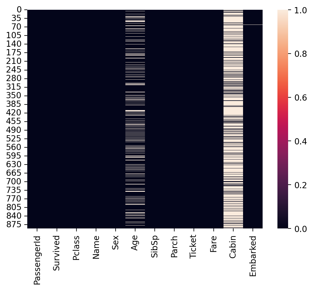
Visualizing missing values

• Finally, we can visualize the rate of missing values across columns using seaborn.heatmap.

  • The dark cells are those with not-null values.

  • The light cells have nan values.

sns.heatmap(df_titanic.isna())

<Axes: >

Step 2: Analyze how the data are distributed

Having identified missing data, the next step is determining how those missing data are distributed.

Is variable \(Y\) different depending on whether \(X\) is nan?

One approach is to ask whether some variable of interest (e.g., Survived) is different depending on whether some other variable is nan.

### Mean survival for people without data about Cabin info
df_titanic[df_titanic['Cabin'].isna()]['Survived'].mean()

0.29985443959243085

### Mean survival for people *with* data about Cabin info
df_titanic[~df_titanic['Cabin'].isna()]['Survived'].mean()

0.6666666666666666

Check-in

What is the mean Survived rate for values with a nan value for Age vs. those with not-null values? How does this compare to the overall Survived rate?

### Your code here

Solution

### Mean survival for people without data about Age
df_titanic[df_titanic['Age'].isna()]['Survived'].mean()

0.2937853107344633

### Mean survival for people *with* data about Age
df_titanic[~df_titanic['Age'].isna()]['Survived'].mean()

0.4061624649859944

### Mean survival for people overall
df_titanic['Survived'].mean()

0.3838383838383838

Additional methods

If you’re interested in diving deeper, you can look into the missingno library in Python (which must be separately installed).

• Tutorial using missingno on a dataset.

• Source code for missingno library.

Step 3: Determine what to do!

Having identified missing data, you need to determine how to handle it.

There are several approaches you can take.

• Removing all rows with any missing data.

• Removing rows with missing data only when that variable is relevant to the analysis or visualization.

• Imputing (i.e., guessing) what values missing data should have.

Removing all rows with any missing data

• We can filter our DataFrame using dropna, which will automatically “drop” any rows containing null values.

• Caution: if you have lots of missing data, this can substantially impact the size of your dataset.

df_filtered = df_titanic.dropna()
df_filtered.shape

(183, 12)

Removing all rows with missing data in specific columns

• Here, we specify that we only want to dropna for rows that have nan in the Age column specifically.

• We still have missing nan for Cabin, but perhaps that’s fine in our case.

df_filtered = df_titanic.dropna(subset = "Age")
df_filtered.shape

(714, 12)

Imputing missing data

One of the most complex (and controversial) approaches is to impute the values of missing data.

There are (again) multiple ways to do this:

1. Decide on a constant value and assign it to all nan values.

   • E.g., assign the mean Age to all people with nan in that column.

2. Try to guess the value based on specific characteristics of the data.

   • E.g., based on other characteristics of this person, what is their likely Age?

Imputing a constant value

We can use fillna to assign all values with nan for Age some other value.

## Assign the mean Age to all people with nan for Age
df_titanic['Age_imputed1'] = df_titanic['Age'].fillna(df_titanic['Age'].mean())
## Now let's look at those rows
df_titanic[df_titanic['Age'].isna()].head(5)

	PassengerId	Survived	Pclass	Name	Sex	Age	SibSp	Parch	Ticket	Fare	Cabin	Embarked	Age_imputed1
5	6	0	3	Moran, Mr. James	male	NaN	0	0	330877	8.4583	NaN	Q	29.699118
17	18	1	2	Williams, Mr. Charles Eugene	male	NaN	0	0	244373	13.0000	NaN	S	29.699118
19	20	1	3	Masselmani, Mrs. Fatima	female	NaN	0	0	2649	7.2250	NaN	C	29.699118
26	27	0	3	Emir, Mr. Farred Chehab	male	NaN	0	0	2631	7.2250	NaN	C	29.699118
28	29	1	3	O'Dwyer, Miss. Ellen "Nellie"	female	NaN	0	0	330959	7.8792	NaN	Q	29.699118

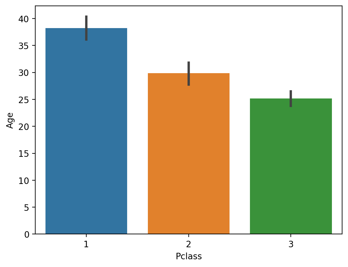
Guessing based on other characteristics

• You can try to guess what their Age would be, based on other features.

• The more sophisticated version of this is to use statistical modeling or using SimpleImputer from the sklearn library.

• For now, simply note that Age correlates with other features (like Pclass).

## Passenger Class is correlated with Age
sns.barplot(data = df_titanic, x = 'Pclass', y = 'Age')

<Axes: xlabel='Pclass', ylabel='Age'>

Check-in

What would happen if you used fillna with the median Age instead of the mean? Why would this matter?

### Your code here

Solution

The median Age is slightly lower.

## Assign the median Age to all people with nan for Age
df_titanic['Age_imputed2'] = df_titanic['Age'].fillna(df_titanic['Age'].median())
## Now let's look at those rows
df_titanic[df_titanic['Age'].isna()].head(5)

	PassengerId	Survived	Pclass	Name	Sex	Age	SibSp	Parch	Ticket	Fare	Cabin	Embarked	Age_imputed1	Age_imputed2
5	6	0	3	Moran, Mr. James	male	NaN	0	0	330877	8.4583	NaN	Q	29.699118	28.0
17	18	1	2	Williams, Mr. Charles Eugene	male	NaN	0	0	244373	13.0000	NaN	S	29.699118	28.0
19	20	1	3	Masselmani, Mrs. Fatima	female	NaN	0	0	2649	7.2250	NaN	C	29.699118	28.0
26	27	0	3	Emir, Mr. Farred Chehab	male	NaN	0	0	2631	7.2250	NaN	C	29.699118	28.0
28	29	1	3	O'Dwyer, Miss. Ellen "Nellie"	female	NaN	0	0	330959	7.8792	NaN	Q	29.699118	28.0

Merging datasets

Merging refers to combining different datasets to leverage the power of additional information.

• In Week 1, we discussed this in the context of data linkage.

• Can link datasets as a function of:

  • Shared time window.

  • Shared identity.

Why merge?

• Each dataset contains limited information.

  • E.g., GDP by Year.

• But merging datasets allows us to see how more variables relate and interact.

• Much of social science research involves locating datasets and figuring out how to combine them.

How to merge?

In Python, pandas.merge allows us to merge two DataFrames on a common column(s).

pd.merge(df1, df2, on = "shared_column")

merge in practice

For demonstration, we’ll merge two Linguistics datasets:

• One dataset contains information about the Age of Acquisition of different English words (Kuperman et al., 2014).

• The other dataset contains information about the Frequency and Concreteness of English words (Brysbaert et al., 2014).

Loading datasets

df_aoa = pd.read_csv("data/wrangling/AoA.csv")
df_aoa.head(1)

	Word	AoA
0	a	2.89

df_conc = pd.read_csv("data/wrangling/concreteness.csv")
df_conc.head(1)

	Word	Concreteness	Frequency	Dom_Pos
0	sled	5.0	149	Adjective

Different kinds of merging

As we see, the datasets are not the same size. This leaves us with a decision to make when merging.

• inner join: Do we preserve only the words in both datasets?

• left join: Do we preserve all the words in one dataset (the “left” one), regardless of whether they occur in the other?

• right join: Do we preserve all the words in one dataset (the “right” one), regardless of whether they occur in the other?

• outer join: Do we preserve all words in both, leaving empty (nan) values where a word only appears in one dataset?

df_aoa.shape

(31124, 2)

df_conc.shape

(28612, 4)

inner join

• For our purposes, it makes the most sense to use an inner join.

• This leaves us with fewer words than occur in either dataset.

df_merged = pd.merge(df_aoa, df_conc, on = "Word", how = "inner")
df_merged.head(2)

	Word	AoA	Concreteness	Frequency	Dom_Pos
0	aardvark	9.89	4.68	21	Noun
1	abacus	8.69	4.52	12	Noun

df_merged.shape

(23569, 5)

Check-in

What happens if you use a different kind of join, e.g., outer or left? What do you notice about the shape of the resulting DataFrame? Do some rows have nan values?

### Your code here

Solution

df_outer_join = pd.merge(df_aoa, df_conc, on = "Word", how = "outer")
df_outer_join.shape

(36167, 5)

df_outer_join.head(4)

	Word	AoA	Concreteness	Frequency	Dom_Pos
0	a	2.89	NaN	NaN	NaN
1	aardvark	9.89	4.68	21.0	Noun
2	abacus	8.69	4.52	12.0	Noun
3	abalone	12.23	NaN	NaN	NaN

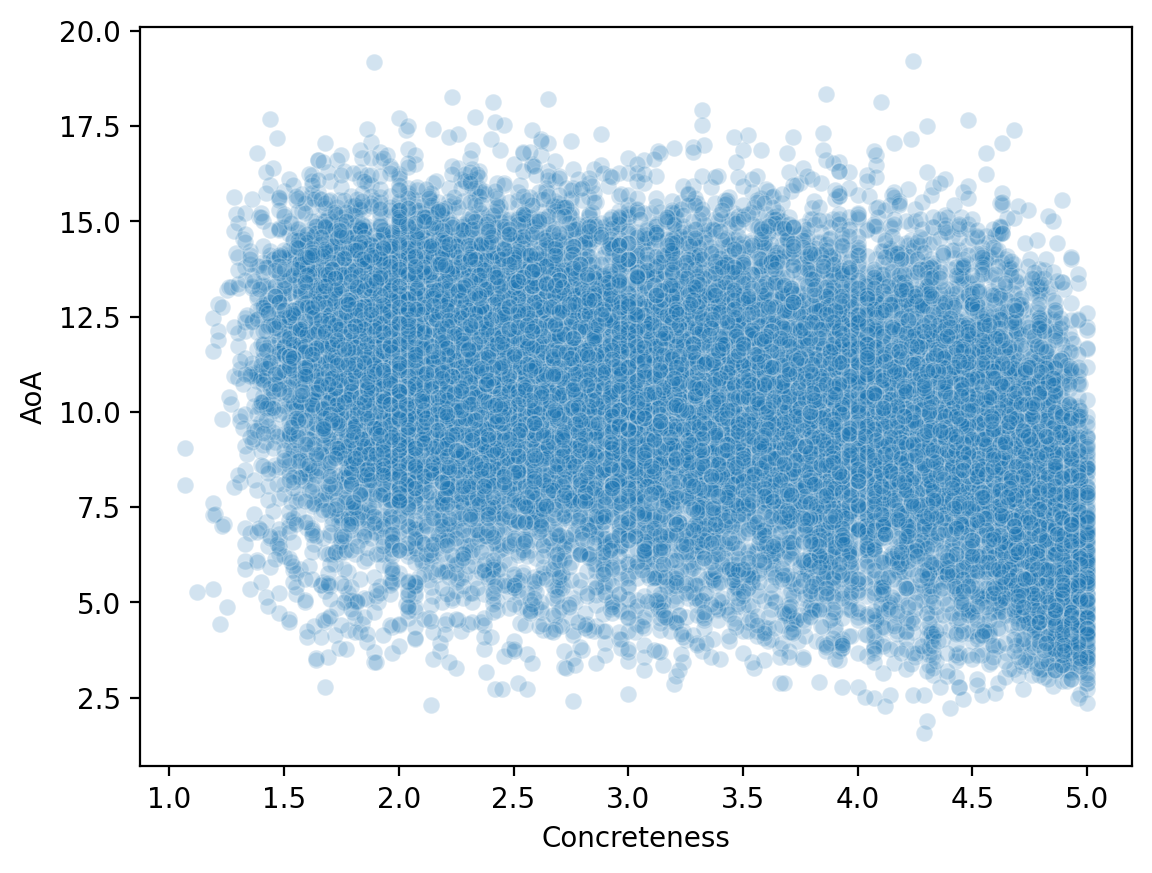
Why merge is so useful

Now that we’ve merged our datasets, we can look at how variables across them relate to each other.

sns.scatterplot(data = df_merged, x = 'Concreteness',
                y = 'AoA', alpha = .2 )

<Axes: xlabel='Concreteness', ylabel='AoA'>

Reshaping data

Reshaping data involves transforming it from one format (e.g., “wide”) to another format (e.g., “long”), to make it more amenable to visualization and analysis.

Often, we need to make our data tidy.

What is tidy data?

Tidy data is a particular way of formatting data, in which:

1. Each variable forms a column (e.g., GDP).

2. Each observation forms a row (e.g., a country).

3. Each type of observational unit forms a table (tabular data!).

Originally developed by Hadley Wickham, creator of the tidyverse in R.

Tidy vs. “untidy” data

Now let’s see some examples of tidy vs. untidy data.

Keep in mind:

• These datasets all contain the same information, just in different formats.

• “Untidy” data can be useful for other things, e.g., presenting in a paper.

• The key goal of tidy data is that each row represents an observation.

Tidy data

Check-in: Why is this data considered tidy?

df_tidy = pd.read_csv("data/wrangling/tidy.csv")
df_tidy

	ppt	condition	rt
0	john	Congruent	200
1	john	Incongruent	250
2	mary	Congruent	178
3	mary	Incongruent	195

Untidy data 1

Check-in: Why is this data not considered tidy?

df_messy1 = pd.read_csv("data/wrangling/messy1.csv")
df_messy1

	john	mary	condition
0	200	178	Congruent
1	250	195	Incongruent

Untidy data 2

Check-in: Why is this data not considered tidy?

df_messy2 = pd.read_csv("data/wrangling/messy2.csv")
df_messy2

	congruent	incongruent	ppt
0	200	250	john
1	178	195	mary

Making data tidy

Fortunately, pandas makes it possible to turn an “untidy” DataFrame into a tidy one.

The key function here is pandas.melt.

pd.melt(df, ### Dataframe
        id_vars = [...], ### what are the identifying columns?
        var_name = ..., ### name for variable grouping over columns
        value_name = ..., ### name for the value this variable takes on

If this seems abstract, don’t worry––it’ll become clearer with examples!

Using pd.melt

• Let’s start with our first messy DataFrame.

• Has columns for each ppt, which contain info about rt.

df_messy1

	john	mary	condition
0	200	178	Congruent
1	250	195	Incongruent

pd.melt(df_messy1, id_vars = 'condition', ### condition is our ID variable
       var_name = 'ppt', ### new row for each ppt observation
       value_name = 'rt') ### label for the info we have about each ppt

	condition	ppt	rt
0	Congruent	john	200
1	Incongruent	john	250
2	Congruent	mary	178
3	Incongruent	mary	195

Check-in

Try to use pd.melt to turn df_messy2 into a tidy DataFrame.

Hint: Think about the existing structure of the DataFrame––how is data grouped––and what the id_vars would be.

df_messy2

	congruent	incongruent	ppt
0	200	250	john
1	178	195	mary

### Your code here

Solution

pd.melt(df_messy2, id_vars = 'ppt', ### here, ppt is our ID variable
       var_name = 'condition', ### new row for each ppt observation
       value_name = 'rt') ### label for the info we have about each ppt

	ppt	condition	rt
0	john	congruent	200
1	mary	congruent	178
2	john	incongruent	250
3	mary	incongruent	195

Hands-on: a real dataset

Now, we’ll turn to a real dataset, which Timothy Lee, creator of Full Stack Economics, compiled and shared with me.

df_work = pd.read_csv("data/viz/missing_work.csv")
df_work.head(5)

	Year	Child care problems	Maternity or paternity leave	Other family or personal obligations	Illness or injury	Vacation	Month
0	2012	18	313	246	899	1701	10
1	2012	35	278	230	880	1299	11
2	2012	13	245	246	944	1005	12
3	2013	14	257	250	1202	1552	1
4	2013	27	258	276	1079	1305	2

Check-in

Is this dataset tidy? How could we make it tidy, if not––i.e., if we wanted each row to be a single observation corresponding to one of the reasons for missing work?

### Your code here

Solution

df_melted = pd.melt(df_work, id_vars = ['Year', 'Month'],
                    var_name = "Reason",
                    value_name = "Days Missed")
df_melted.head(2)

	Year	Month	Reason	Days Missed
0	2012	10	Child care problems	18
1	2012	11	Child care problems	35

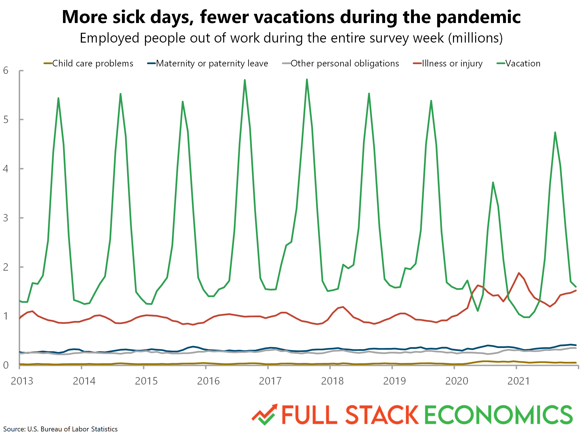
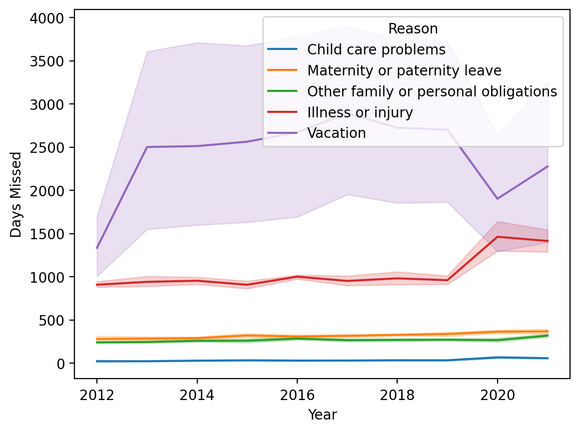
Why tidy data is useful

Finally, let’s use this dataset to recreate a graph from FullStackEconomics.

Original graph

Check-in

As a first-pass approach, what tools from seaborn could you use to recreate this plot?

### Your code here

Solution

This is okay, but not really what we want. This is grouping it by Year. But we want to group by both Year and Month.

sns.lineplot(data = df_melted, x = 'Year', y = 'Days Missed', hue = "Reason")

<Axes: xlabel='Year', ylabel='Days Missed'>

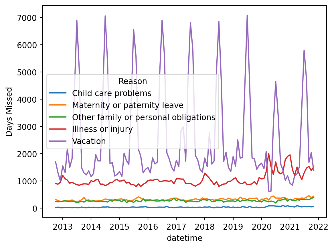
Using datetime

• Let’s make a new column called date, which combines the Month and Year.

• Then we can use pd.to_datetime to turn that into a custom pandas representation.

## First, let's concatenate each month and year into a single string
df_melted['date'] = df_melted.apply(lambda row: str(row['Month']) + '-' + str(row['Year']), axis = 1)
df_melted.head(2)

	Year	Month	Reason	Days Missed	date
0	2012	10	Child care problems	18	10-2012
1	2012	11	Child care problems	35	11-2012

## Now, let's create a new "datetime" column using the `pd.to_datetime` function
df_melted['datetime'] = pd.to_datetime(df_melted['date'])
df_melted.head(2)

/var/folders/pn/5zbmv0cj31v6hmyh53njhmdw0000gn/T/ipykernel_1691/714386078.py:2: UserWarning: Could not infer format, so each element will be parsed individually, falling back to `dateutil`. To ensure parsing is consistent and as-expected, please specify a format.
  df_melted['datetime'] = pd.to_datetime(df_melted['date'])

	Year	Month	Reason	Days Missed	date	datetime
0	2012	10	Child care problems	18	10-2012	2012-10-01
1	2012	11	Child care problems	35	11-2012	2012-11-01

Plotting again

Much better!

sns.lineplot(data = df_melted, x = "datetime", y = "Days Missed", hue = "Reason")

<Axes: xlabel='datetime', ylabel='Days Missed'>

Conclusion

This was an introduction to data wrangling.

• As noted, data wrangling is a hugely important topic––and could constitute an entire class.

• But today, we’ve focused on:

  • Identifying and addressing missing data.

  • Merging datasets.

  • Making data tidy.