Logistic Regression#
Libraries#
## Imports
import pandas as pd
import numpy as np
import matplotlib.pyplot as plt
import statsmodels.api as sm
import statsmodels.formula.api as smf
import seaborn as sns
import scipy.stats as ss
%matplotlib inline
%config InlineBackend.figure_format = 'retina'  # makes figs nicer!
Goals of this lecture#
Introduction to classification.
Foundations of logistic regression.
“Generalizing” the linear model.
Log-odds and the logistic function.
Implementing logistic regression in
statsmodels.
What is classification?#
In statistical modeling, classification refers the problem of predicting a categorical response variable \(Y\) using some set of features \(X\).
There are many examples of categorical responses:
Is an email
spamornot spam?Is a cell mass
cancerornot cancer?Will this customer
buyornot buythe product?Is a credit card
fraudulentornot fraudulent?Is this a picture of a
cat, adog, aperson, orother?
Before we discuss how to do this, it’s important to reflect on what exactly a “category” is.
“To classify is human”#
“To classify is human…We sort dirty dishes from clean, white laundry from colorfast, important email to be answered from e-junk…. Any part of the home, school, or workplace reveals some such system of classification: medications classed as not for children occupy a higher shelf than safer ones; books for reference are shelved close to where we do the Sunday crossword puzzle; door keys are color-coded and stored according to frequency of use.”
-Bowker & Star, 2000
We often impose a category structure onto the world––as needed––and these categories in turn can have real impact on our lives.
E.g., whether a behavior is diagnosed as a
mental illness.E.g., whether the census includes multiple options for
ethnicity.
Check-in#
What aspects of your life involve category structure? Which ones do you think have the “right” category structure, and why do you think that?
Categories and the problem of measurement#
The issue of which categories are “correct” is an instance of more general questions around measurement and construct validity.
As we discuss the practical task of classifying data, there are important questions to keep in mind:
Where is the boundary drawn between categories?
Who decides the category structure?
What function do these categories serve?
What variance is obscured by these categories? What is illuminated?
And remember that the map is not the territory.
How many categories?#
One question is how many categories there are.
Binary classification involves sorting inputs \(X\) into one of two labels.
E.g.,
spamvs.not spam.
But many classification tasks involve more than two labels.
E.g., face recognition involves \(N\) categories, where \(N =\) number of possible identities.
Foundations of logistic regression#
Logistic regression is a widely used approach for modeling binary, categorical data.
To understand logistic regression, we’ll have to dive into the theoretical foundations of the logistic function.
Example dataset: spam#
As we learn logistic regression, we’ll start with a dataset about different emails, with information about which ones were considered spam.
df_spam = pd.read_csv("data/models/classification/email.csv")
df_spam.head(3)
| spam | to_multiple | from | cc | sent_email | time | image | attach | dollar | winner | ... | viagra | password | num_char | line_breaks | format | re_subj | exclaim_subj | urgent_subj | exclaim_mess | number | |
|---|---|---|---|---|---|---|---|---|---|---|---|---|---|---|---|---|---|---|---|---|---|
| 0 | 0 | 0 | 1 | 0 | 0 | 2012-01-01T06:16:41Z | 0 | 0 | 0 | no | ... | 0 | 0 | 11.370 | 202 | 1 | 0 | 0 | 0 | 0 | big |
| 1 | 0 | 0 | 1 | 0 | 0 | 2012-01-01T07:03:59Z | 0 | 0 | 0 | no | ... | 0 | 0 | 10.504 | 202 | 1 | 0 | 0 | 0 | 1 | small |
| 2 | 0 | 0 | 1 | 0 | 0 | 2012-01-01T16:00:32Z | 0 | 0 | 4 | no | ... | 0 | 0 | 7.773 | 192 | 1 | 0 | 0 | 0 | 6 | small |
3 rows × 21 columns
Why not linear regression?#
The spam variable is coded as 0 (no) or 1 (yes).
In principle, we could treat this a continuous variable, and model
spamusing linear regression.We could interpret our prediction \(\hat{y}\) as the probability of the outcome.
Does anyone see any issues with this?
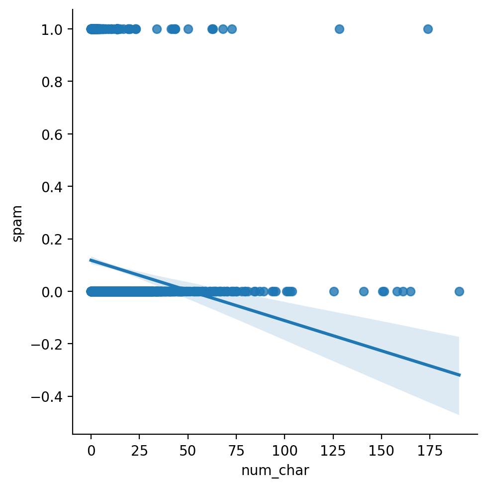
Going beyond \([0, 1]\)#
A linear model will generate predictions beyond \([0, 1]\), even though probability should be bounded at \([0, 1]\).
sns.lmplot(data = df_spam, x = "num_char", y = "spam")
/Users/seantrott/anaconda3/lib/python3.11/site-packages/seaborn/axisgrid.py:118: UserWarning: The figure layout has changed to tight
  self._figure.tight_layout(*args, **kwargs)
<seaborn.axisgrid.FacetGrid at 0x135c857d0>
Framing the problem probabilistically#
We want to sort input into different labels, so it’s helpful to think of this probabilistically.
Treat each outcome as Bernoulli trials, i.e., “success” (
spam) and “failure” (not spam).Each observation has an independent probability of success, \(p_i\).
On its own, this is just be the proportion of spam emails, i.e., \(p(spam)\).
Our goal is to model \(p_i\) conditioned on other variables that might relate to \(p_i\).
Check-in#
On its own, \(p_i\) is just the probability of success (e.g., spam). What does this remind you of from linear regression?
Solution#
On its own, the probability of success is most analogous to an Intercept-only model in linear regression––i.e., the mean of \(Y\).
Generalizing the linear model (GLMs)#
Generalized linear models (GLMs) are generalizations of linear regression.
Each GLM has:
A probability distribution representing the generative model for the outcome variable.
A linear model: \(\eta = \beta_0 + \beta_1X_1 + ... + \beta_nX_n\)
A link function relating the linear model to the outcome we’re interested in.
We can design a function that links the linear model to a probability score, i.e., \([0, 1]\).
Quick tour of GLMs#
There are many different kinds of generalized linear models. Some of the most common are:
Model name |
Distribution |
Link name |
Use cases |
Example |
|---|---|---|---|---|
Ordinary linear regression |
Normal distribution |
Identity |
Linear response data |
|
Logistic regression |
Bernoulli/Binomial |
Binary response data |
|
|
Poisson regression |
Poisson |
Count data |
|
We’ll be focusing on logistic regression.
Logistic regression#
Logistic regression uses a logit link function.
\(\Large logit(p) = log(\frac{p}{1 - p})\)
Where \(p\) is the probability of some outcome.
Takes a value between \([0, 1]\) and maps it to a value between \([-\infty, \infty]\).
Also called the log odds.
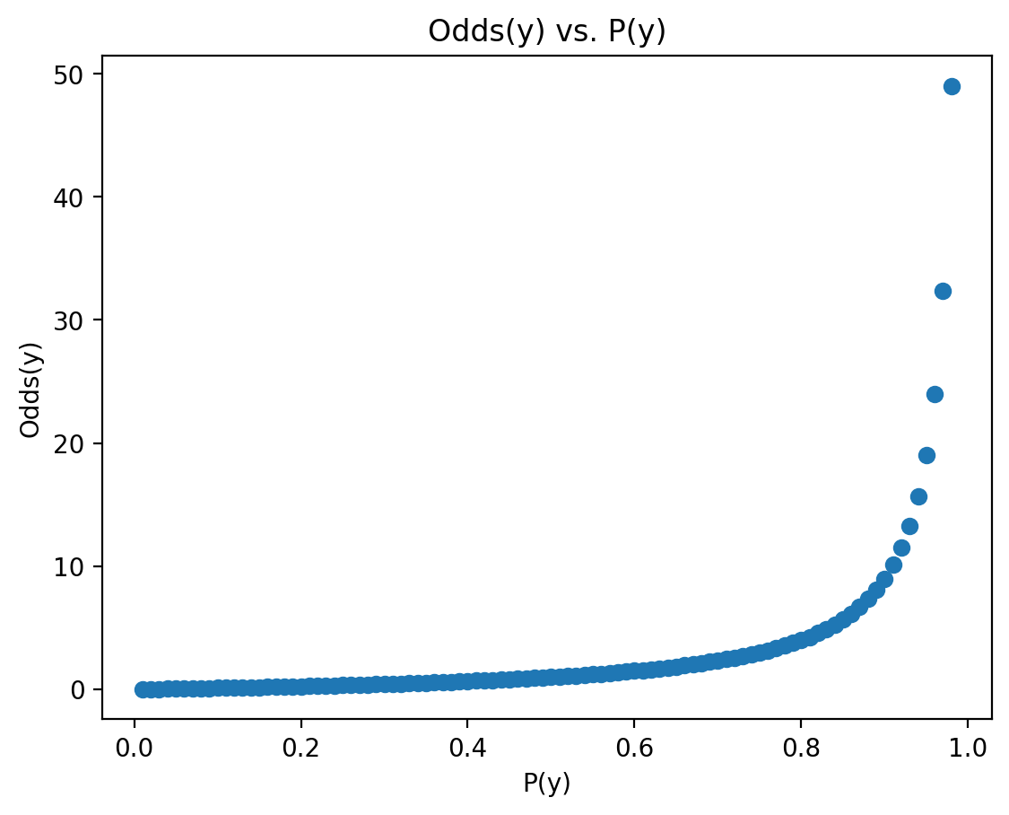
Introducing the odds#
The odds of an event are the ratio of the probability of the event occurring, \(p(y)\), to the probability of the event not occuring, \(1 - p(y)\).
\(Odds(p) = \Large \frac{p}{1 - p}\)
Unlike \(p\), the odds are bounded at \([0, \infty]\).
p = np.arange(.01, .99, .01)
odds = p / (1 - p)
plt.scatter(p, odds)
plt.xlabel("P(y)")
plt.ylabel("Odds(y)")
plt.title("Odds(y) vs. P(y)")
Text(0.5, 1.0, 'Odds(y) vs. P(y)')
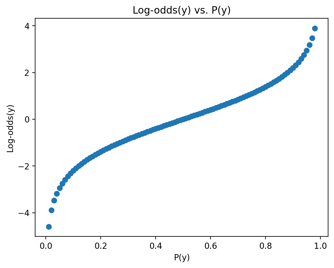
Introducing the log-odds#
The log-odds of an event is the log of the odds of that event. This is also called the logit function.
\(Logit(p) = log(\frac{p}{1 - p})\)
Unlike \(p\), the log-odds are bounded at \([-\infty, \infty]\).
lo = np.log(p / (1 - p))
plt.scatter(p, lo)
plt.xlabel("P(y)")
plt.ylabel("Log-odds(y)")
plt.title("Log-odds(y) vs. P(y)")
Text(0.5, 1.0, 'Log-odds(y) vs. P(y)')
Check-in#
Would the log-odds of \(p(y) = .6\) be positive or negative?
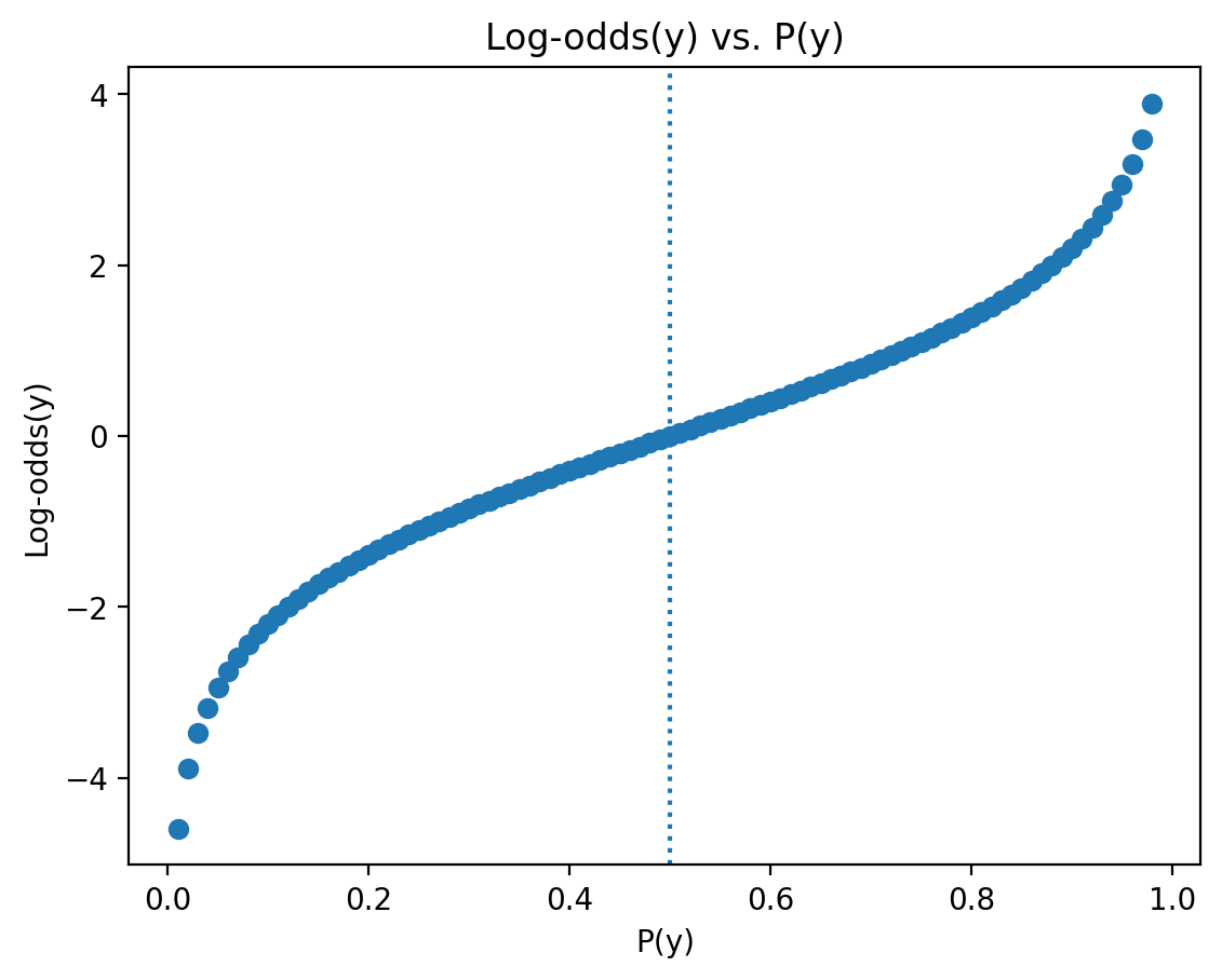
Interpreting the sign of log-odds#
The sign of log-odds can be interpreted as reflecting whether \(p(y) > .5\) (positive) or \(p(y) < .5\) (negative).
plt.scatter(p, lo)
plt.xlabel("P(y)")
plt.ylabel("Log-odds(y)")
plt.title("Log-odds(y) vs. P(y)")
plt.axvline(x = .5, linestyle = "dotted")
<matplotlib.lines.Line2D at 0x1363e1c10>
Check-in#
Is log-odds(y) linearly related to p(y)? Why does this matter?
A non-linear relationship#
The log-odds of \(y\) is non-linearly related to the probability of \(y\).
This means that we can’t interpret linear changes in log-odds as linear changes in probability.
That will be very important when we build logistic regression models.
Introducing the logistic function#
The logistic function is the inverse of the logit function. It converts the log-odds back to probability.
The logistic function is defined as:
\(\Large \frac{e^x}{1 + e^x}\)
Where \(x\) is the log-odds of an event.
Check-in#
Would applying the logistic function to a log-odds of 1 yield a \(p >.5\) or \(p < .5\)?
### Your code here
Mapping from log-odds to \(p\)#
We can use np.exp(x) to compute \(e^x\).
lo = 1
p = np.exp(lo) / (np.exp(lo) + 1)
p ### p is > .5
0.7310585786300049
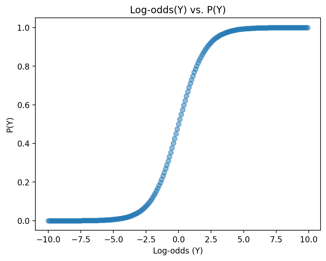
A more general mapping#
log_odds = np.arange(-10, 10, .1)
p = np.exp(log_odds) / (1 + np.exp(log_odds))
plt.scatter(log_odds, p, alpha = .5)
plt.xlabel("Log-odds (Y)")
plt.ylabel("P(Y)")
plt.title("Log-odds(Y) vs. P(Y)")
Text(0.5, 1.0, 'Log-odds(Y) vs. P(Y)')
Where does regression come into play?#
With logistic regression, we learn parameters \(\beta_0, ..., \beta_n\) for the following equation:
\(\Large log(\frac{p}{1 - p}) = \beta_0 + \beta_1X_1 + \epsilon\)
Our “dependent variable” is technically the log-odds (logit) of \(p\).
Thus, we are learning a linear relationship between \(X\) and the log-odds of our outcome.
Check-in#
Based on this formulation:
\(log(\frac{p}{1 - p}) = \beta_0 + \beta_1X_1 + \epsilon\)
How would we interpret \(\beta_1 = 1\) with respect to log odds?
Log-odds ~ \(X\) is linear#
There is a straightforward linear interpretation between our parameters \(\beta_0, ..., \beta_n\) and the log-odds of our outcome.
That is, if \(\beta_1=1\):
For each 1-unit increase in \(X\), the log-odds of our outcome increases by \(1\).
If \(\beta_1 = 2\):
For each 1-unit increase in \(X\), the log-odds of our outcome increases by \(2\).
Check-in#
Based on this formulation:
\(log(\frac{p}{1 - p}) = \beta_0 + \beta_1X_1 + \epsilon\)
How would we interpret \(\beta_1 = 1\) with respect to probability?
\(p\) ~\(X\) is not linear#
The mapping between log-odds and \(p(y)\) is not linear.
This means that we can’t interpret our coefficients linearly with respect to \(p\).
log_odds = np.arange(-10, 10, .1)
p = np.exp(log_odds) / (1 + np.exp(log_odds))
plt.scatter(log_odds, p, alpha = .5)
plt.xlabel("Log-odds (Y)")
plt.ylabel("P(Y)")
plt.title("Log-odds(Y) vs. P(Y)")
Text(0.5, 1.0, 'Log-odds(Y) vs. P(Y)')
Logistic regression in Python#
To perform logistic regression in Python, we can use the statsmodels package, which has the logit method.
smf.logit(data = df_name, formula = "y ~ x").fit()
Fitting the models is relatively straightforward––the hard(er) part is interpreting them.
Fitting the model#
To start, let’s fit a model predicting spam from num_char (i.e., how long the message is).
mod_len = smf.logit(data = df_spam, formula = "spam ~ num_char").fit()
mod_len.summary()
Optimization terminated successfully.
         Current function value: 0.299210
         Iterations 8
| Dep. Variable: | spam | No. Observations: | 3921 |
|---|---|---|---|
| Model: | Logit | Df Residuals: | 3919 |
| Method: | MLE | Df Model: | 1 |
| Date: | Fri, 12 Jan 2024 | Pseudo R-squ.: | 0.03725 |
| Time: | 10:40:32 | Log-Likelihood: | -1173.2 |
| converged: | True | LL-Null: | -1218.6 |
| Covariance Type: | nonrobust | LLR p-value: | 1.607e-21 |
| coef | std err | z | P>|z| | [0.025 | 0.975] | |
|---|---|---|---|---|---|---|
| Intercept | -1.7987 | 0.072 | -25.135 | 0.000 | -1.939 | -1.658 |
| num_char | -0.0621 | 0.008 | -7.746 | 0.000 | -0.078 | -0.046 |
Interpreting the model#
In this simple model, we can interpret the coefficients as follows:
Intercept: the log-odds of an email beingspamwhennum_char == 0.num_char: for every 1-unit increase innum_char, how does the log-odds of an email beingspamchange?
\(Y = -1.8 - 0.06*X_{length} + \epsilon\)
mod_len.params
Intercept   -1.798738
num_char    -0.062071
dtype: float64
Check-in#
Based on these coefficients, what is the predicted probability of an utterance being spam when num_char == 0?
### Your code here
Deriving \(p\) using logistic function#
To calculate \(p(y)\), we need to convert log-odds back to probability.
log_odds = -1.8 # Just the intercept
p = np.exp(log_odds) / (1 + np.exp(log_odds))
p
0.1418510649004878
Check-in#
Based on these coefficients, what is the predicted probability of an utterance being spam when num_char == 100?
### Your code here
Deriving \(p\) (pt. 2)#
Here, we need to:
Calculate log-odds by inputting \(X\) into the equation.
Convert log-odds back to probability using the logistic function.
log_odds = -1.8 - 0.06 * 100
p = np.exp(log_odds) / (1 + np.exp(log_odds))
p
0.00040956716498605043
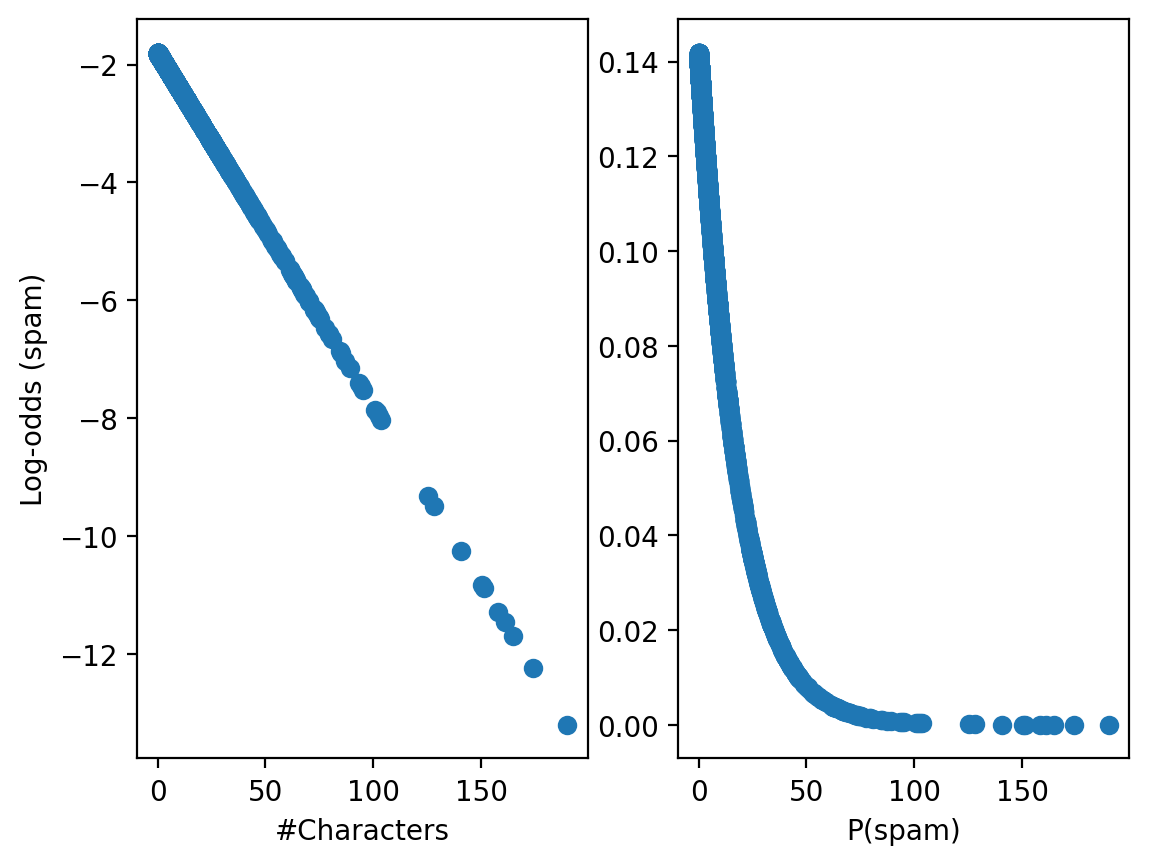
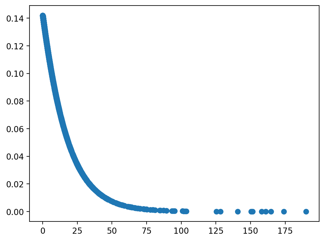
Log-odds != probability#
X = df_spam['num_char']
lo = -1.8 - .06 * X
p = np.exp(lo) / (1 + np.exp(lo))
fig, axes = plt.subplots(1, 2)
axes[0].scatter(X, lo)
axes[1].scatter(X, p)
axes[0].set_xlabel("#Characters")
axes[1].set_xlabel("#Characters")
axes[0].set_ylabel("Log-odds (spam)")
axes[1].set_xlabel("P(spam)")
Text(0.5, 0, 'P(spam)')
Logistic regression with categorical predictors#
Instead of using num_char (a continuous predictor), we can use a categorical predictor (like winner: whether or not an email has the word “winner”).
mod_winner = smf.logit(data = df_spam, formula = "spam ~ winner").fit()
mod_winner.summary()
Optimization terminated successfully.
         Current function value: 0.307661
         Iterations 6
| Dep. Variable: | spam | No. Observations: | 3921 |
|---|---|---|---|
| Model: | Logit | Df Residuals: | 3919 |
| Method: | MLE | Df Model: | 1 |
| Date: | Fri, 12 Jan 2024 | Pseudo R-squ.: | 0.01005 |
| Time: | 10:40:32 | Log-Likelihood: | -1206.3 |
| converged: | True | LL-Null: | -1218.6 |
| Covariance Type: | nonrobust | LLR p-value: | 7.410e-07 |
| coef | std err | z | P>|z| | [0.025 | 0.975] | |
|---|---|---|---|---|---|---|
| Intercept | -2.3140 | 0.056 | -41.121 | 0.000 | -2.424 | -2.204 |
| winner[T.yes] | 1.5256 | 0.275 | 5.538 | 0.000 | 0.986 | 2.066 |
Check-in#
How should we interpret the parameters of this model?
### Your code here
Interpreting \(\beta\) for categorical predictors#
As with linear regression, the \(\beta\) for a categorical predictor means predicted change in log-odds relative to the Intercept
Here, \(\beta_0\) is the predicted log-odds when
winner == no.$\beta_1 is the predicted change in log-odds (relative to the
Intercept) whenwinner == yes.
mod_winner.params
Intercept       -2.314047
winner[T.yes]    1.525589
dtype: float64
Check-in#
According to the model, what is \(p(spam)\) for emails that don’t have the word winner?
### Your code here
Solution#
lo = mod_winner.params['Intercept']
np.exp(lo) / (np.exp(lo) + 1)
0.0899662950479635
Check-in#
According to the model, what is \(p(spam)\) for emails that do have the word winner?
### Your code here
Solution#
lo = mod_winner.params['Intercept'] + mod_winner.params['winner[T.yes]']
np.exp(lo) / (np.exp(lo) + 1)
0.31249999999999994
Generating predictions#
By default, predict() will generate predicted \(p\).
plt.scatter(df_spam['num_char'], mod_len.predict())
<matplotlib.collections.PathCollection at 0x13664b390>
Conclusion#
Many use-cases of statistical modeling involve a categorical response variable.
Logistic regression can be used for binary classication tasks.
Logistic regression is a generalized linear model (GLM).
Predicts the log-odds of \(Y\) as a linear function of \(X\).
Log-odds can be converted to \(p\) using the logistic function.