Unsupervised clustering

Libraries

## Imports
import pandas as pd
import numpy as np
import matplotlib.pyplot as plt
import seaborn as sns
import scipy.stats as ss

%matplotlib inline
%config InlineBackend.figure_format = 'retina'  # makes figs nicer!

Goals of this lecture

• Introducing unsupervised approaches: dealing with unlabeled data.

• Finding structure with K-means clustering.

Unsupervised approaches: an introduction

Broadly, statistical modeling approaches can be either:

• Supervised: learn from some function \(f\) mapping features to labels (\(Y\)) \(X\) t\(Y\).

• Unsupervised: learning some function \(f\) finding structure in features, without labels.

So far, all the models we’ve discussed (e.g., linear regression, logistic regression), have been supervised.

Why unsupervised learning?

In unsupervised learning, a model learns patterns from unlabeled data.

This is useful for a few reasons:

• It’s practical: doesn’t require defining or acquiring labels for data.

• It’s conceptually interesting: humans (arguably) don’t have direct, supervised feedback.

  • Labels or categories often emerge from exposure to data––they don’t exist a priori.

• It’s helpful: unsupervised approaches help identify structure in a dataset.

  • Useful for exploratory data analysis.

The challenge of unsupervised learning

Supervised learning is straightforward:

• Clear goal: predict \(Y\) from \(X\).

• Clear evaluation metric: how well did we predict \(Y\)?

Unsupervised learning is harder to define:

• What is our goal?

• How do we check our work?

Unsupervised learning in action

Despite these challenges, unsupervised learning is of growing importance to computational researchers.

Many examples of its use:

• Clustering cells on their gene expressions to identify different cancer subtypes.

• Identify groups of shoppers based on shopping habits to develop different advertising schemes.

• Clustering word uses (e.g., “river bank” vs. “financial bank”) to identify distinct meanings.

Clustering

Clustering refers to any approach towards finding sub-groups (i.e., “clusters”) in a dataset.

Basic goal:

• Put observations \(x_i\) and \(x_j\) in the same cluster if similar.

• Put observations \(x_i\) and \(x_j\) in different clusters if they are different.

Of course, this requires defining what makes two observations similar or different.

Introducing \(K\)-means clustering

K-means clustering is a clustering approach that aims to partition \(n\) observations into \(k\) non-overlapping clusters.

Ideally, we would like to do this in a way that minimizes within-cluster variation.

Check-in: What’s one intuitive way we could define within-cluster variation?

Defining within-cluster variation

A simple way to define within-cluster variation is as follows:

\(\Large \frac{1}{n}*\sum_i(x_i - \bar{x_i})^2\)

This is the average squared distance of each point from the mean of that cluster.

Basic intuition:

• A “good” cluster is one with low variance.

• A “bad” cluster is one which has high variance.

The \(K\)-means algorithm

There are many ways to partition \(n\) points into \(k\) groups.

The \(K\)-means algorithm gives us a “local optimum”––not perfect, but pretty good.

• Start by determining desired number of clusters (\(k\)).

• Then, randomly assign each observation to a random cluster \(k\).

• Now, iterate until the cluster assignment stops changing…

  • For each cluster \(k\), compute the centroid (the mean)

  • Assign each observation to the cluster whose centroid is closest (using Euclidean distance).

After many iterations, this algorithm converges onto a locally optimal solution.

\(K\)-means in practice

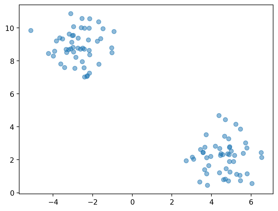
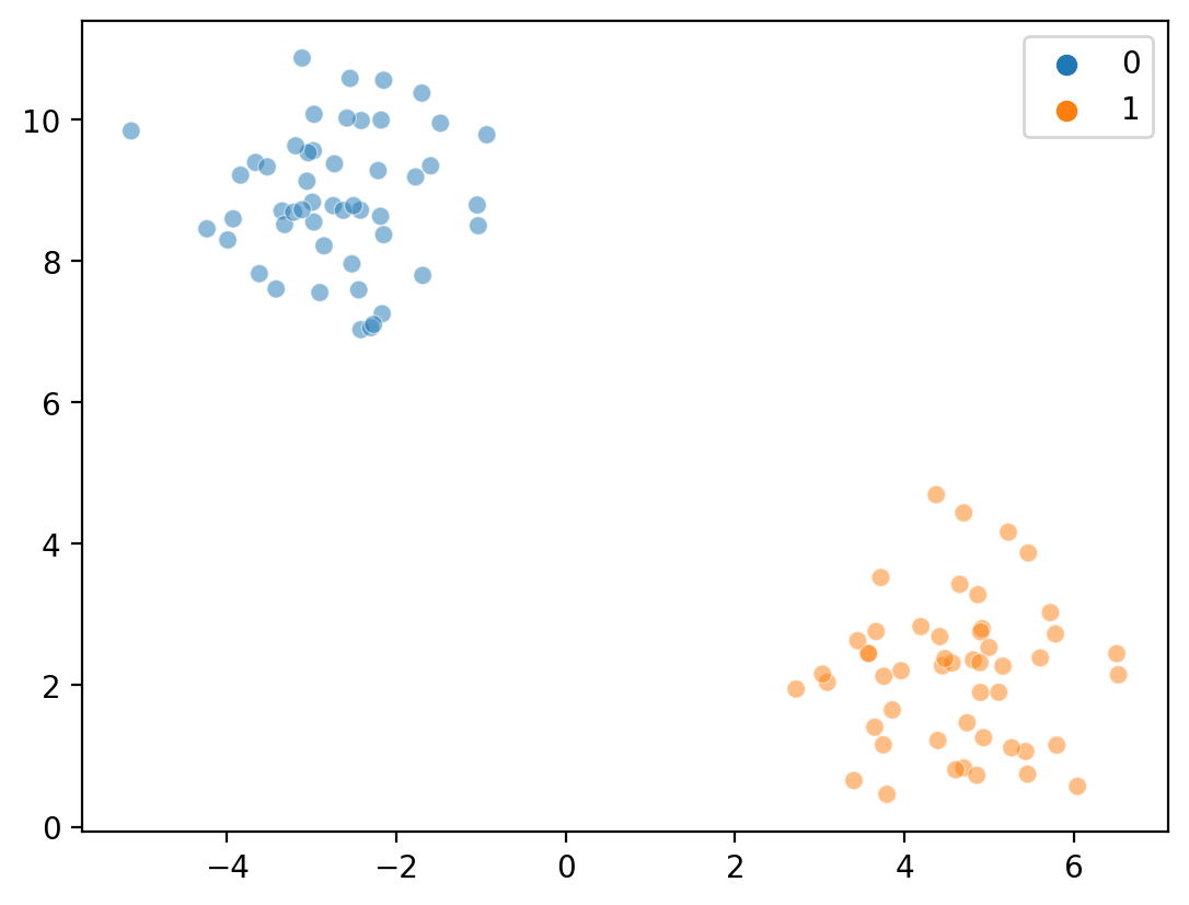
To illustrate \(K\)-means, we’ll code it from scratch. First, we’ll generate a small dataset for demonstration purposes.

from sklearn.datasets import make_blobs ### easy way to make clusters

X, y = make_blobs(n_samples=100, centers=2, random_state=42)
plt.scatter(X[:, 0], X[:, 1], alpha = .5)

<matplotlib.collections.PathCollection at 0x1607753d0>

Step 1: determine \(K\)

• The first step is determining the number of clusters.

• This is not a trivial step––but one approach is to start small, e.g., \(K = 2\).

  • Ideally, we could test multiple values of \(K\), and test which is optimal.

Let’s set \(K = 2\).

K = 2

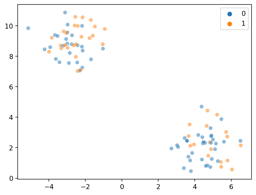
Step 2: Randomly assign points to clusters

Now, we randomly assign either a 0 or a 1 to each point.

labels = np.random.randint(K, size = len(X))
sns.scatterplot(x = X[:, 0], y = X[:, 1], hue = labels, alpha = .5)

<Axes: >

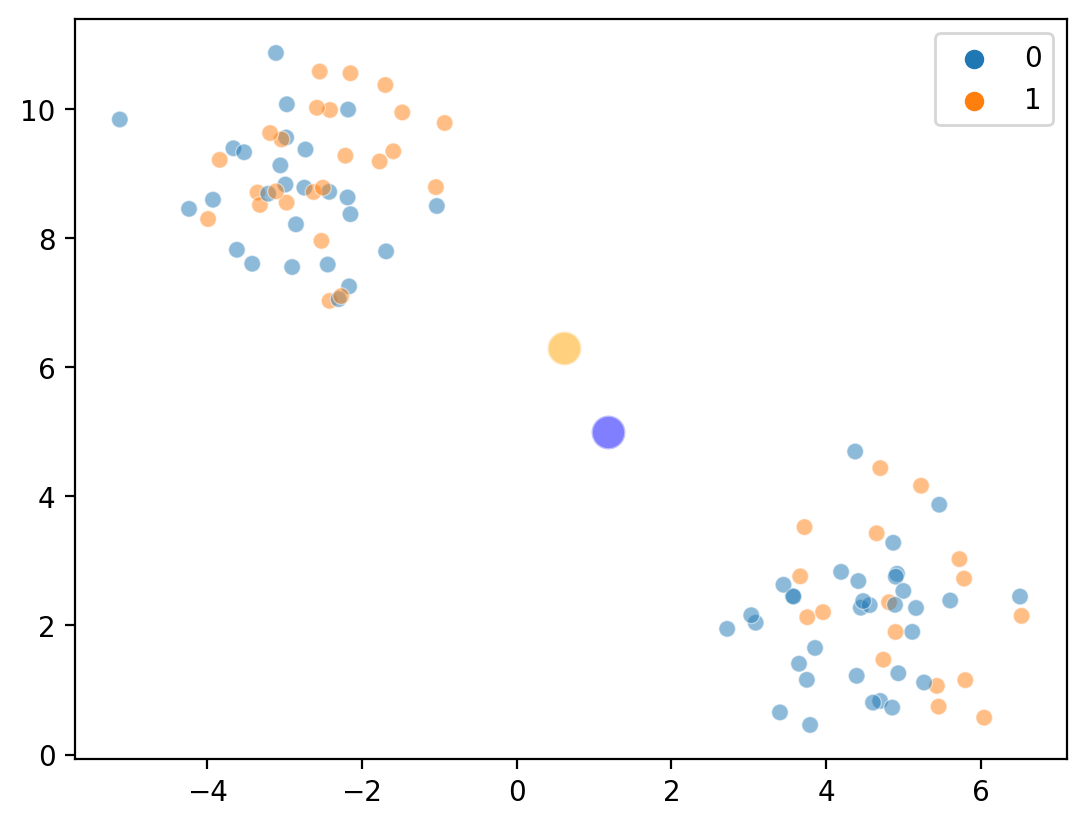
Step 3a: Calculate cluster centroids

Now, we compute the average of points randomly assigning to \(K = 0\) vs. \(K = 1\).

c1_mean = X[labels==0].mean(axis=0)
c2_mean = X[labels==1].mean(axis=0)
print("Cluster 1 mean: {x}".format(x = c1_mean))
print("Cluster 2 mean: {x}".format(x = c2_mean))

Cluster 1 mean: [1.18530246 4.99421035]
Cluster 2 mean: [0.61807869 6.30113252]

Overlaying cluster centroids…

sns.scatterplot(x = X[:, 0], y = X[:, 1], hue = labels, alpha = .5)
sns.scatterplot(x = [c1_mean[0]], y = [c1_mean[1]], color = "blue", s = 150, alpha = .5)
sns.scatterplot(x = [c2_mean[0]], y = [c2_mean[1]], color = "orange", s = 150, alpha = .5)
# sns.scatterplot(x = c2_mean[0], y = c2_mean[1], hue = "orange", s = 100)

<Axes: >

Step 3b: reassign points

Now, we reassign points to the nearest cluster centroid.

from scipy.spatial.distance import euclidean

d_c1 = [euclidean(i, c1_mean)**2 for i in X]
d_c2 = [euclidean(i, c2_mean)**2 for i in X]

new_labels = []
for index, point in enumerate(X):
    ### compare distance to c1 vs. c2
    if d_c1[index] < d_c2[index]:
        new_labels.append(0)
    else:
        new_labels.append(1)
new_labels = np.array(new_labels)

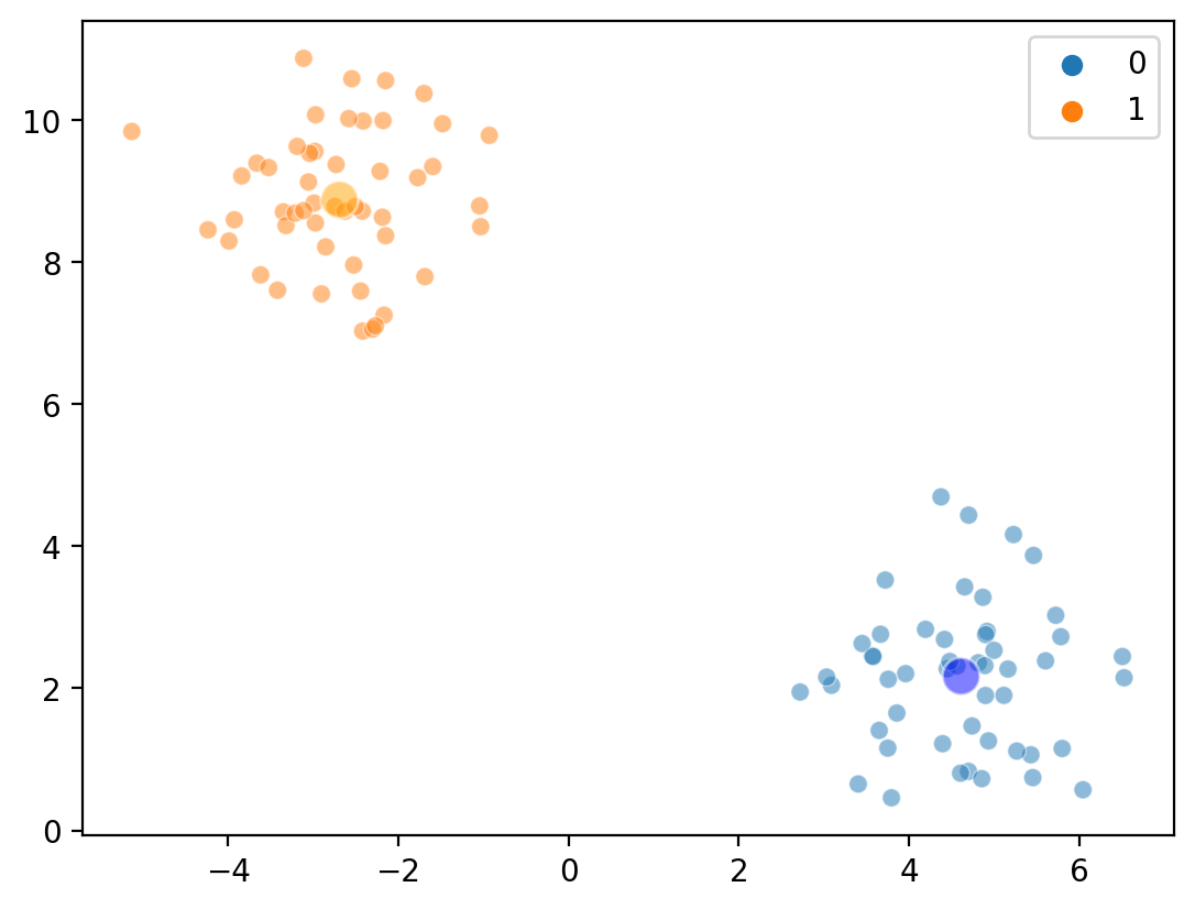
Step 3a: Re-compute centroids

c1_mean = X[new_labels==0].mean(axis=0)
c2_mean = X[new_labels==1].mean(axis=0)
print("Cluster 1 mean: {x}".format(x = c1_mean))
print("Cluster 2 mean: {x}".format(x = c2_mean))

Cluster 1 mean: [4.60840443 2.16998192]
Cluster 2 mean: [-2.70292301  8.89011496]

Overlaying cluster centroids (again)

Within one iteration, we’ve sorted our points into very distinct clusters!

sns.scatterplot(x = X[:, 0], y = X[:, 1], hue = new_labels, alpha = .5)
sns.scatterplot(x = [c1_mean[0]], y = [c1_mean[1]], color = "blue", s = 150, alpha = .5)
sns.scatterplot(x = [c2_mean[0]], y = [c2_mean[1]], color = "orange", s = 150, alpha = .5)
# sns.scatterplot(x = c2_mean[0], y = c2_mean[1], hue = "orange", s = 100)

<Axes: >

\(K\)-means with sklearn

Fortunately, you won’t need to code the \(K\)-means algorithm by hand. The sklearn package has a KMeans algorithm built-in.

KMeans(n_clusters = ### decide k
       n_iter = ### number of iterations
       ...)

Steps to using KMeans:

1. Import and instantiate the KMeans class.

2. Use fit_predict on X to fit the algorithm and generate labels.

from sklearn.cluster import KMeans

Replicating analysis with KMeans

k = KMeans(n_clusters = K)
kmeans_labels = k.fit_predict(X)

/Users/seantrott/anaconda3/lib/python3.11/site-packages/sklearn/cluster/_kmeans.py:1412: FutureWarning: The default value of `n_init` will change from 10 to 'auto' in 1.4. Set the value of `n_init` explicitly to suppress the warning
  super()._check_params_vs_input(X, default_n_init=10)

sns.scatterplot(x = X[:, 0], y = X[:, 1], hue = kmeans_labels, alpha = .5)

<Axes: >

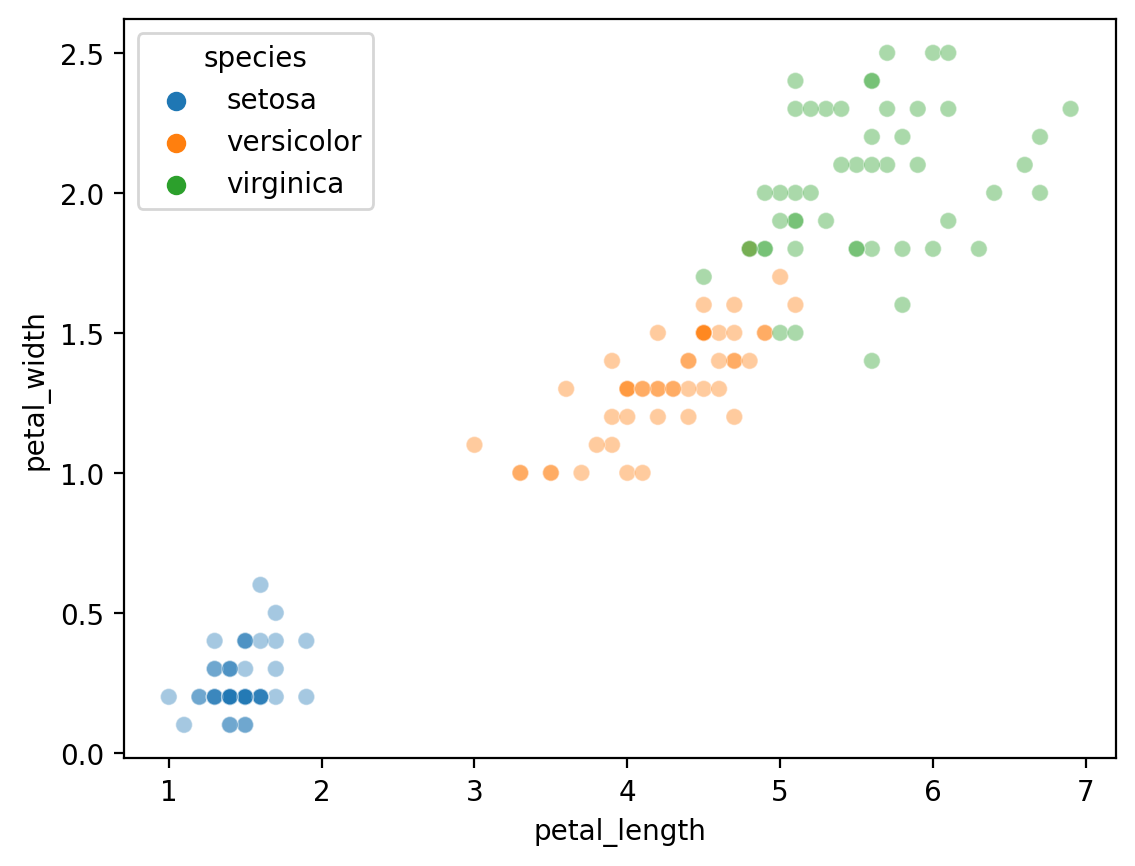
Applying to the iris dataset

Now, we will apply KMeans to the famous iris dataset.

• Our goal will be to cluster the dataset…

• … then see whether the clusters correspond to the true species labels.

df_iris = sns.load_dataset("iris")
sns.scatterplot(data = df_iris, x = "petal_length", y = "petal_width", hue = "species", alpha = .4)

<Axes: xlabel='petal_length', ylabel='petal_width'>

Check-in

Apply KMeans with k = 2 to the iris dataset (focusing on the features below), then visualize your clusters. What does it look like?

features = df_iris[['petal_length', 'petal_width']].values
### Your code here

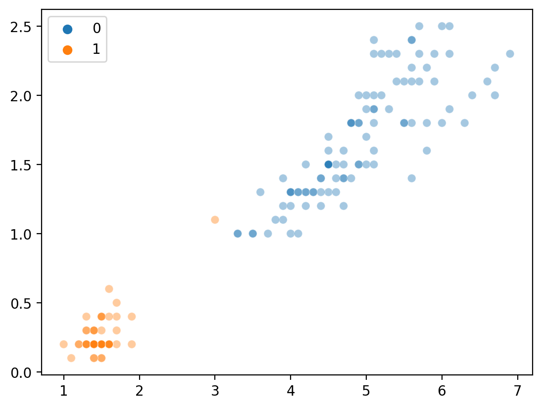
Clustering with \(K = 2\)

Not bad––although we know that species = 3, so it’s obviously not perfect.

new_labels = KMeans(n_clusters = 2).fit_predict(features)
sns.scatterplot(x = features[:,0], y = features[:, 1], hue = new_labels, alpha = .4)

/Users/seantrott/anaconda3/lib/python3.11/site-packages/sklearn/cluster/_kmeans.py:1412: FutureWarning: The default value of `n_init` will change from 10 to 'auto' in 1.4. Set the value of `n_init` explicitly to suppress the warning
  super()._check_params_vs_input(X, default_n_init=10)

<Axes: >

Clustering with \(K = 3\)

Much better.

new_labels = [str(i) for i in KMeans(n_clusters = 3).fit_predict(features)]
sns.scatterplot(x = features[:,0], y = features[:, 1], hue = new_labels, alpha = .4)

/Users/seantrott/anaconda3/lib/python3.11/site-packages/sklearn/cluster/_kmeans.py:1412: FutureWarning: The default value of `n_init` will change from 10 to 'auto' in 1.4. Set the value of `n_init` explicitly to suppress the warning
  super()._check_params_vs_input(X, default_n_init=10)

<Axes: >

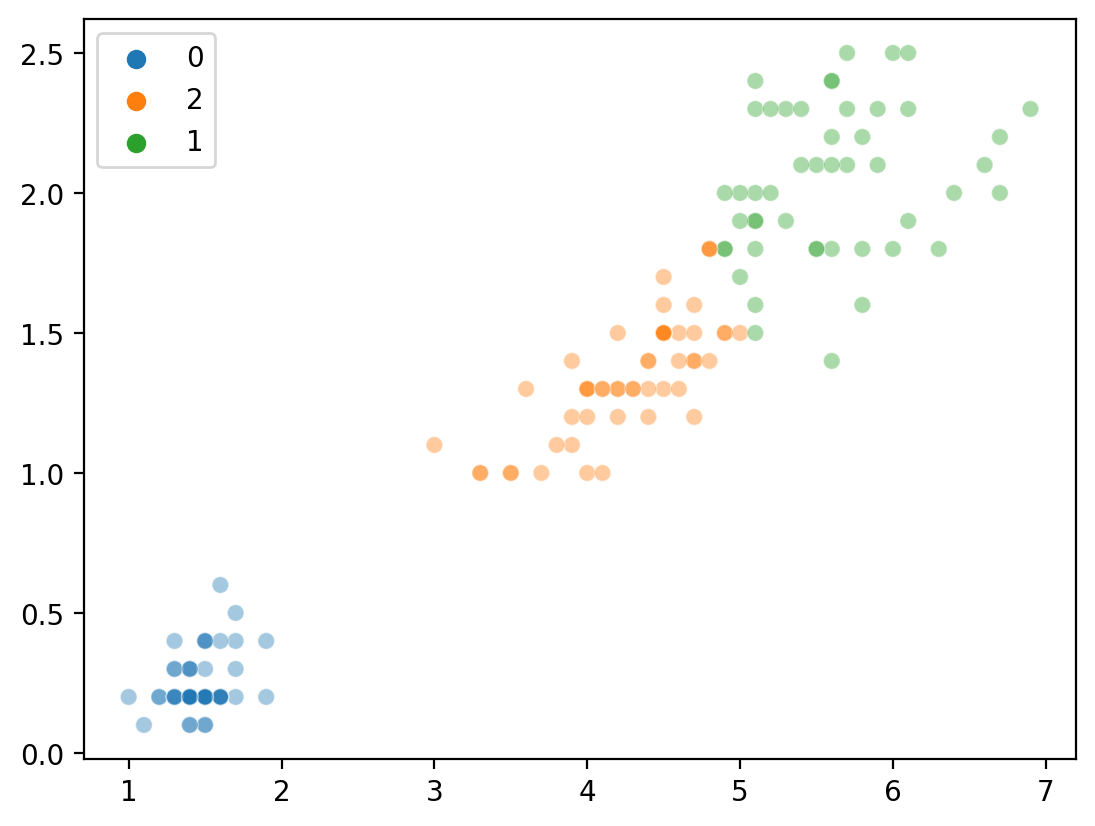
How did we do?

We can ask whether our cluster labels correspond to the true category structure of species using a technique called the adjusted rand score.

• The Rand Index computes a similarity measure between two clusterings of the same data, ranging from \([0, 1]\).

• The adjusted rand score adjusts for the performance you’d expect by chance.

from sklearn.metrics import adjusted_rand_score

adjusted_rand_score(new_labels, df_iris['species'])

0.8856970310281228

Determining the optimal \(K\)

A major challenge with K-means clustering is determining the “right” value of \(K\).

• If we know the true number of categories, we can set \(K\) to that.

  • However, we rarely know this in practice.

• Additionally, we’d like our method to be able to find the optimal \(K\) in an unsupervised fashion as well.

There are many different approaches to determining the optimal \(K\)––still an active area of machine learning research.

Conceptual issue: lumpers vs. splitters

Without “ground truth” labels, a set of observations could be described with very few or very many clusters.

• Minimum number of clusters: \(K = 2\).

• Maximum number of clusters: \(K = n\), where \(n\) is number of observations.

Lumpers vs. splitters: Some people (“lumpers”) favor a smaller number of clusters; others (“splitters”) favor fine classification distinctions.

splitters make very small units – their critics say that if they can tell two animals apart, they place them in different genera … and if they cannot tell them apart, they place them in different species. … Lumpers make large units – their critics say that if a carnivore is neither a dog nor a bear, they call it a cat. (Simpson, 1945)

Approach 1: Elbow method

The “elbow method” is an approach for determining the optimal clusters \(K\), which involves identifying the smallest value of \(K\) that significantly reduces within-cluster variation.

Basic intuition:

• Accuracy: We want a set of clusters that reduce within-cluster variation as much as possible.

• Parsimony: We don’t want too many clusters.

  • \(K = n\) would have 0 within-cluster variance, but wouldn’t be very useful!

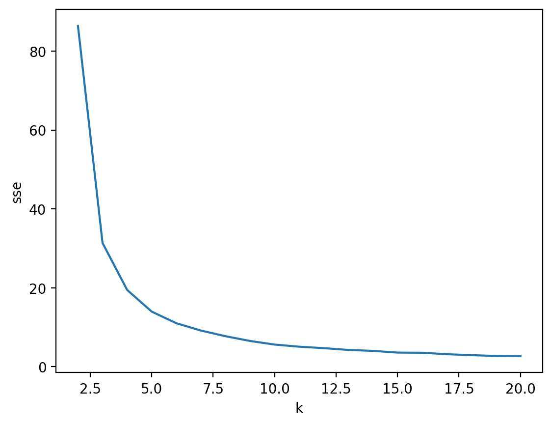
Elbow method in practice (pt. 1)

The average within-cluster variation can be accessed for a given KMeans model using the inertia_ attribute.

sse = []
for k in range(2, 21):
    km = KMeans(n_clusters = k).fit(features)
    sse.append({'k': k, 'sse': km.inertia_})

/Users/seantrott/anaconda3/lib/python3.11/site-packages/sklearn/cluster/_kmeans.py:1412: FutureWarning: The default value of `n_init` will change from 10 to 'auto' in 1.4. Set the value of `n_init` explicitly to suppress the warning
  super()._check_params_vs_input(X, default_n_init=10)
/Users/seantrott/anaconda3/lib/python3.11/site-packages/sklearn/cluster/_kmeans.py:1412: FutureWarning: The default value of `n_init` will change from 10 to 'auto' in 1.4. Set the value of `n_init` explicitly to suppress the warning
  super()._check_params_vs_input(X, default_n_init=10)
/Users/seantrott/anaconda3/lib/python3.11/site-packages/sklearn/cluster/_kmeans.py:1412: FutureWarning: The default value of `n_init` will change from 10 to 'auto' in 1.4. Set the value of `n_init` explicitly to suppress the warning
  super()._check_params_vs_input(X, default_n_init=10)
/Users/seantrott/anaconda3/lib/python3.11/site-packages/sklearn/cluster/_kmeans.py:1412: FutureWarning: The default value of `n_init` will change from 10 to 'auto' in 1.4. Set the value of `n_init` explicitly to suppress the warning
  super()._check_params_vs_input(X, default_n_init=10)

/Users/seantrott/anaconda3/lib/python3.11/site-packages/sklearn/cluster/_kmeans.py:1412: FutureWarning: The default value of `n_init` will change from 10 to 'auto' in 1.4. Set the value of `n_init` explicitly to suppress the warning
  super()._check_params_vs_input(X, default_n_init=10)
/Users/seantrott/anaconda3/lib/python3.11/site-packages/sklearn/cluster/_kmeans.py:1412: FutureWarning: The default value of `n_init` will change from 10 to 'auto' in 1.4. Set the value of `n_init` explicitly to suppress the warning
  super()._check_params_vs_input(X, default_n_init=10)
/Users/seantrott/anaconda3/lib/python3.11/site-packages/sklearn/cluster/_kmeans.py:1412: FutureWarning: The default value of `n_init` will change from 10 to 'auto' in 1.4. Set the value of `n_init` explicitly to suppress the warning
  super()._check_params_vs_input(X, default_n_init=10)
/Users/seantrott/anaconda3/lib/python3.11/site-packages/sklearn/cluster/_kmeans.py:1412: FutureWarning: The default value of `n_init` will change from 10 to 'auto' in 1.4. Set the value of `n_init` explicitly to suppress the warning
  super()._check_params_vs_input(X, default_n_init=10)
/Users/seantrott/anaconda3/lib/python3.11/site-packages/sklearn/cluster/_kmeans.py:1412: FutureWarning: The default value of `n_init` will change from 10 to 'auto' in 1.4. Set the value of `n_init` explicitly to suppress the warning
  super()._check_params_vs_input(X, default_n_init=10)
/Users/seantrott/anaconda3/lib/python3.11/site-packages/sklearn/cluster/_kmeans.py:1412: FutureWarning: The default value of `n_init` will change from 10 to 'auto' in 1.4. Set the value of `n_init` explicitly to suppress the warning
  super()._check_params_vs_input(X, default_n_init=10)
/Users/seantrott/anaconda3/lib/python3.11/site-packages/sklearn/cluster/_kmeans.py:1412: FutureWarning: The default value of `n_init` will change from 10 to 'auto' in 1.4. Set the value of `n_init` explicitly to suppress the warning
  super()._check_params_vs_input(X, default_n_init=10)

/Users/seantrott/anaconda3/lib/python3.11/site-packages/sklearn/cluster/_kmeans.py:1412: FutureWarning: The default value of `n_init` will change from 10 to 'auto' in 1.4. Set the value of `n_init` explicitly to suppress the warning
  super()._check_params_vs_input(X, default_n_init=10)
/Users/seantrott/anaconda3/lib/python3.11/site-packages/sklearn/cluster/_kmeans.py:1412: FutureWarning: The default value of `n_init` will change from 10 to 'auto' in 1.4. Set the value of `n_init` explicitly to suppress the warning
  super()._check_params_vs_input(X, default_n_init=10)
/Users/seantrott/anaconda3/lib/python3.11/site-packages/sklearn/cluster/_kmeans.py:1412: FutureWarning: The default value of `n_init` will change from 10 to 'auto' in 1.4. Set the value of `n_init` explicitly to suppress the warning
  super()._check_params_vs_input(X, default_n_init=10)

/Users/seantrott/anaconda3/lib/python3.11/site-packages/sklearn/cluster/_kmeans.py:1412: FutureWarning: The default value of `n_init` will change from 10 to 'auto' in 1.4. Set the value of `n_init` explicitly to suppress the warning
  super()._check_params_vs_input(X, default_n_init=10)
/Users/seantrott/anaconda3/lib/python3.11/site-packages/sklearn/cluster/_kmeans.py:1412: FutureWarning: The default value of `n_init` will change from 10 to 'auto' in 1.4. Set the value of `n_init` explicitly to suppress the warning
  super()._check_params_vs_input(X, default_n_init=10)
/Users/seantrott/anaconda3/lib/python3.11/site-packages/sklearn/cluster/_kmeans.py:1412: FutureWarning: The default value of `n_init` will change from 10 to 'auto' in 1.4. Set the value of `n_init` explicitly to suppress the warning
  super()._check_params_vs_input(X, default_n_init=10)
/Users/seantrott/anaconda3/lib/python3.11/site-packages/sklearn/cluster/_kmeans.py:1412: FutureWarning: The default value of `n_init` will change from 10 to 'auto' in 1.4. Set the value of `n_init` explicitly to suppress the warning
  super()._check_params_vs_input(X, default_n_init=10)
/Users/seantrott/anaconda3/lib/python3.11/site-packages/sklearn/cluster/_kmeans.py:1412: FutureWarning: The default value of `n_init` will change from 10 to 'auto' in 1.4. Set the value of `n_init` explicitly to suppress the warning
  super()._check_params_vs_input(X, default_n_init=10)

df = pd.DataFrame(sse)
df.head(1)

	k	sse
0	2	86.39022

Elbow method in practice (pt. 2)

The elbow (or “knee”) is the point at which a curve visibly bends.

Based on these results, the optimal \(K\) is between 3-5.

sns.lineplot(data = df, x = 'k', y = 'sse')

<Axes: xlabel='k', ylabel='sse'>

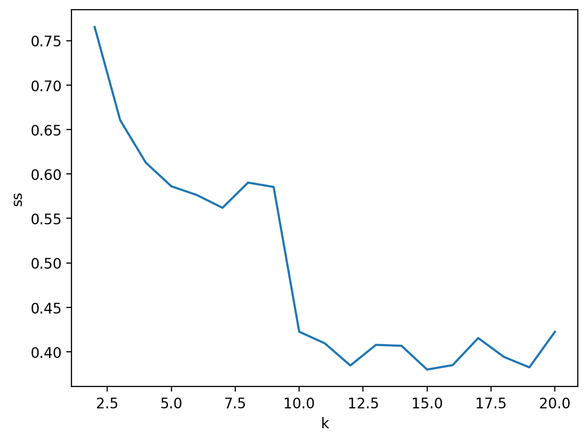
Approach 2: Silhouette analysis

Silhouette analysis measures the difference between each point’s distance from all points in other clusters and each point’s distance from all points in the same clusters.

• The silhouette score ranges from -1 (very bad) to 1 (very good).

• Like \(SSE\), this will capture the amount of within-cluster variance.

• Unlike \(SSE\), it also rewards distant clusters.

That is: Minimize within-cluster distance, maximize across-cluster distance.

Silhouette analysis in sklearn (pt. 1)

from sklearn.metrics import silhouette_score

ss = []
for k in range(2, 21):
    new_labels = KMeans(n_clusters = k).fit_predict(features)
    ss.append({'k': k, 'ss': silhouette_score(features, new_labels)})
df = pd.DataFrame(ss)
df.head(1)

/Users/seantrott/anaconda3/lib/python3.11/site-packages/sklearn/cluster/_kmeans.py:1412: FutureWarning: The default value of `n_init` will change from 10 to 'auto' in 1.4. Set the value of `n_init` explicitly to suppress the warning
  super()._check_params_vs_input(X, default_n_init=10)

/Users/seantrott/anaconda3/lib/python3.11/site-packages/sklearn/cluster/_kmeans.py:1412: FutureWarning: The default value of `n_init` will change from 10 to 'auto' in 1.4. Set the value of `n_init` explicitly to suppress the warning
  super()._check_params_vs_input(X, default_n_init=10)
/Users/seantrott/anaconda3/lib/python3.11/site-packages/sklearn/cluster/_kmeans.py:1412: FutureWarning: The default value of `n_init` will change from 10 to 'auto' in 1.4. Set the value of `n_init` explicitly to suppress the warning
  super()._check_params_vs_input(X, default_n_init=10)
/Users/seantrott/anaconda3/lib/python3.11/site-packages/sklearn/cluster/_kmeans.py:1412: FutureWarning: The default value of `n_init` will change from 10 to 'auto' in 1.4. Set the value of `n_init` explicitly to suppress the warning
  super()._check_params_vs_input(X, default_n_init=10)
/Users/seantrott/anaconda3/lib/python3.11/site-packages/sklearn/cluster/_kmeans.py:1412: FutureWarning: The default value of `n_init` will change from 10 to 'auto' in 1.4. Set the value of `n_init` explicitly to suppress the warning
  super()._check_params_vs_input(X, default_n_init=10)
/Users/seantrott/anaconda3/lib/python3.11/site-packages/sklearn/cluster/_kmeans.py:1412: FutureWarning: The default value of `n_init` will change from 10 to 'auto' in 1.4. Set the value of `n_init` explicitly to suppress the warning
  super()._check_params_vs_input(X, default_n_init=10)

/Users/seantrott/anaconda3/lib/python3.11/site-packages/sklearn/cluster/_kmeans.py:1412: FutureWarning: The default value of `n_init` will change from 10 to 'auto' in 1.4. Set the value of `n_init` explicitly to suppress the warning
  super()._check_params_vs_input(X, default_n_init=10)

/Users/seantrott/anaconda3/lib/python3.11/site-packages/sklearn/cluster/_kmeans.py:1412: FutureWarning: The default value of `n_init` will change from 10 to 'auto' in 1.4. Set the value of `n_init` explicitly to suppress the warning
  super()._check_params_vs_input(X, default_n_init=10)
/Users/seantrott/anaconda3/lib/python3.11/site-packages/sklearn/cluster/_kmeans.py:1412: FutureWarning: The default value of `n_init` will change from 10 to 'auto' in 1.4. Set the value of `n_init` explicitly to suppress the warning
  super()._check_params_vs_input(X, default_n_init=10)
/Users/seantrott/anaconda3/lib/python3.11/site-packages/sklearn/cluster/_kmeans.py:1412: FutureWarning: The default value of `n_init` will change from 10 to 'auto' in 1.4. Set the value of `n_init` explicitly to suppress the warning
  super()._check_params_vs_input(X, default_n_init=10)
/Users/seantrott/anaconda3/lib/python3.11/site-packages/sklearn/cluster/_kmeans.py:1412: FutureWarning: The default value of `n_init` will change from 10 to 'auto' in 1.4. Set the value of `n_init` explicitly to suppress the warning
  super()._check_params_vs_input(X, default_n_init=10)

/Users/seantrott/anaconda3/lib/python3.11/site-packages/sklearn/cluster/_kmeans.py:1412: FutureWarning: The default value of `n_init` will change from 10 to 'auto' in 1.4. Set the value of `n_init` explicitly to suppress the warning
  super()._check_params_vs_input(X, default_n_init=10)

/Users/seantrott/anaconda3/lib/python3.11/site-packages/sklearn/cluster/_kmeans.py:1412: FutureWarning: The default value of `n_init` will change from 10 to 'auto' in 1.4. Set the value of `n_init` explicitly to suppress the warning
  super()._check_params_vs_input(X, default_n_init=10)
/Users/seantrott/anaconda3/lib/python3.11/site-packages/sklearn/cluster/_kmeans.py:1412: FutureWarning: The default value of `n_init` will change from 10 to 'auto' in 1.4. Set the value of `n_init` explicitly to suppress the warning
  super()._check_params_vs_input(X, default_n_init=10)
/Users/seantrott/anaconda3/lib/python3.11/site-packages/sklearn/cluster/_kmeans.py:1412: FutureWarning: The default value of `n_init` will change from 10 to 'auto' in 1.4. Set the value of `n_init` explicitly to suppress the warning
  super()._check_params_vs_input(X, default_n_init=10)
/Users/seantrott/anaconda3/lib/python3.11/site-packages/sklearn/cluster/_kmeans.py:1412: FutureWarning: The default value of `n_init` will change from 10 to 'auto' in 1.4. Set the value of `n_init` explicitly to suppress the warning
  super()._check_params_vs_input(X, default_n_init=10)

/Users/seantrott/anaconda3/lib/python3.11/site-packages/sklearn/cluster/_kmeans.py:1412: FutureWarning: The default value of `n_init` will change from 10 to 'auto' in 1.4. Set the value of `n_init` explicitly to suppress the warning
  super()._check_params_vs_input(X, default_n_init=10)
/Users/seantrott/anaconda3/lib/python3.11/site-packages/sklearn/cluster/_kmeans.py:1412: FutureWarning: The default value of `n_init` will change from 10 to 'auto' in 1.4. Set the value of `n_init` explicitly to suppress the warning
  super()._check_params_vs_input(X, default_n_init=10)

/Users/seantrott/anaconda3/lib/python3.11/site-packages/sklearn/cluster/_kmeans.py:1412: FutureWarning: The default value of `n_init` will change from 10 to 'auto' in 1.4. Set the value of `n_init` explicitly to suppress the warning
  super()._check_params_vs_input(X, default_n_init=10)

	k	ss
0	2	0.76539

Silhouette analysis in sklearn (pt. 2)

Unlike with \(SSE\), the silhouette score does not monotonically improve as \(K\) increases.

sns.lineplot(data = df, x = "k", y = "ss")

<Axes: xlabel='k', ylabel='ss'>

Limitations of \(K\)-means

As with any model, \(K\)-means has a number of limitations, including:

• You must choose \(K\) manually, and there’s no “perfect” method for choosing the right \(K\).

• It’s dependent on your random_state (global optimum is not guaranteed).

• It’s sensitive to outliers, which will affect the centroid of a cluster.

• In “vanilla” formulation, does not handle clusters of different sizes or shapes.

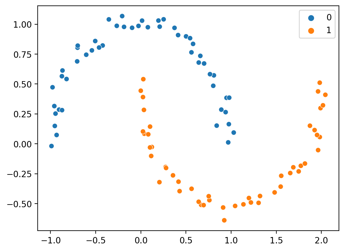
Clusters aren’t always spheroidal!

from sklearn.datasets import make_moons

X, y = make_moons(n_samples=100, noise = .05)
sns.scatterplot(x = X[:, 0], y = X[:, 1], hue = y)

<Axes: >

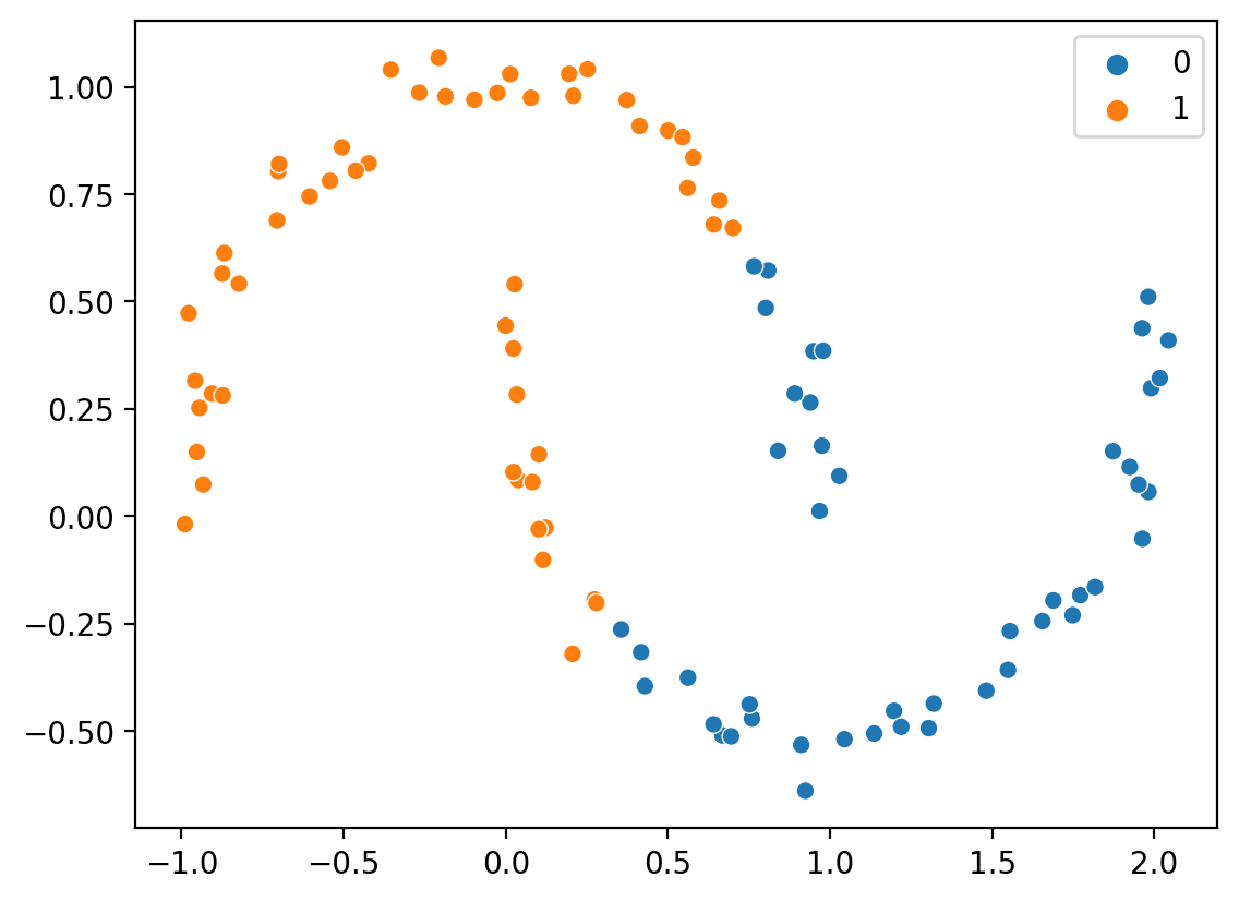
KMeans falters with non-spheroidal data

k = KMeans(n_clusters=2)
new_labels = k.fit_predict(X)
sns.scatterplot(x = X[:, 0], y = X[:, 1], hue = new_labels)

/Users/seantrott/anaconda3/lib/python3.11/site-packages/sklearn/cluster/_kmeans.py:1412: FutureWarning: The default value of `n_init` will change from 10 to 'auto' in 1.4. Set the value of `n_init` explicitly to suppress the warning
  super()._check_params_vs_input(X, default_n_init=10)

<Axes: >

Clustering beyond \(K\)-means

There are many algorithms for unsupervised clustering:

• Hierarchical clustering: iteratively join pairs of points into clusters, then group clusters together, and so on.

• Gaussian mixture model: tries to estimate \(K\) latent Gaussian functions responsible for generating data.

  • Can be used as a more flexible, general form of K-means.

• DBSCAN: density-based spatial clustering of applications with noise.

  • Unlike K-means, does not require specification of \(K\), and can fit more flexible cluster shapes.

Conclusion

• Unsupervised learning is an integral part of computational social science.

• One approach is clustering, which involves sorting \(n\) data points into \(k\) groups.

• K-means clustering is an iterative algorithm that:

  • Given some value of \(K\)…

  • … tends to find the clusters that reduce within-cluster variation.

• The elbow method and silhouette analysis are two approaches to evaluating your clusters.