Linear regression: prediction error and more#
Libraries#
## Imports
import pandas as pd
import numpy as np
import matplotlib.pyplot as plt
import statsmodels.api as sm
import statsmodels.formula.api as smf
import seaborn as sns
import scipy.stats as ss
%matplotlib inline
%config InlineBackend.figure_format = 'retina'  # makes figs nicer!
Goals of this lecture#
Extracting model predictions.
Basic model evaluation:
Visualizing \(\hat{Y}\) vs. \(Y\).
\(RSS\): residual sum of squares.
\(S_{Y|X}\): standard error of the estimate.
Using \(S_{Y|X}\) to calculate standard error for our coefficients.
\(R^2\): coefficient of determination.
Homoscedasticity.
Models as predictors#
Modeling our data#
A statistical model is a mathematical model representing a “data-generating process”.
This means we can use a model to generate predictions for some value of \(X\).
\(\Large \hat{Y} = f(X, \beta)\)
df_income = pd.read_csv("data/models/income.csv")
df_income.head(3)
| Education | Seniority | Income | |
|---|---|---|---|
| 0 | 21.586207 | 113.103448 | 99.917173 |
| 1 | 18.275862 | 119.310345 | 92.579135 |
| 2 | 12.068966 | 100.689655 | 34.678727 |
Predictions from a linear model#
Predictions from a linear model can be obtained by “plugging in” some value of \(X\) to the linear equation with fit model parameters (\(\beta_0\), \(\beta_1\)).
mod_edu = smf.ols(data = df_income, formula = "Income ~ Education").fit()
mod_edu.params
Intercept   -41.916612
Education     6.387161
dtype: float64
Here, the linear equation would be written:
\(Y = -41.92 + 6.39 * X_1 + \epsilon\)
X = 10
-41.92 + 6.39 * X ## predicted income when X = 10
21.979999999999997
Predictions using statsmodels#
Instead of generating predictions by hand, you can use the
predictfunction instatsmodels.By default, this will generate predictions for all of the original values of \(X\).
mod_edu.predict()
array([95.95797131, 74.81426521, 35.16981627, 66.88537542, 85.38611826,
       74.81426521, 85.38611826, 93.31500804, 88.02908152, 21.95499996,
       45.74166932, 77.45722847, 32.52685301, 64.24241216, 21.95499996,
       88.02908152, 48.38463259, 64.24241216, 64.24241216, 88.02908152,
       74.81426521, 51.02759585, 69.52833868, 24.59796322, 95.95797131,
       29.88388975, 85.38611826, 32.52685301, 35.16981627, 66.88537542])
predict() for new data?#
You can also use predict() for new data––it just needs to be represented as a DataFrame with the appropriate columns.
## Create new DataFrame
new_data = pd.DataFrame({'Education': [10, 25, 35]})
mod_edu.predict(new_data)
0     21.955000
1    117.762418
2    181.634030
dtype: float64
Model evaluation#
Once we’ve built a model, we want to evaluate it: how good is this model?
We’ll discuss several ways to evaluate our linear model:
Visually: plotting \(\hat{Y}\) or the residuals of the model.
Evaluation metrics: \(RSS\), \(MSE\), and \(S_{Y|X}\)
Visual comparisons#
We can use data visualizations to evaluate the success of our model.
There are a few ways to do this:
Plotting \(\hat{Y}\) as the regression line over
IncomeandEducation.Directly plotting \(\hat{Y}\) vs. \(Y\).
Plotting the residuals of our model.
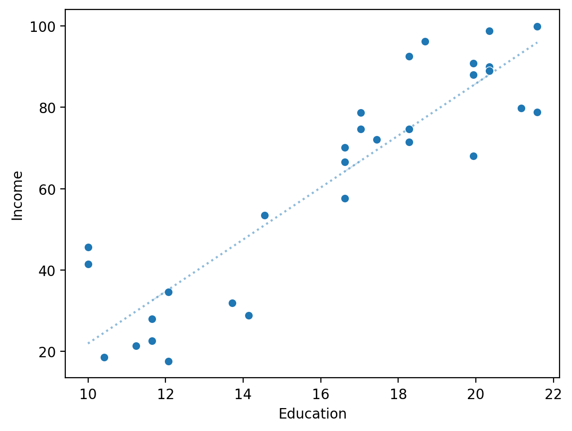
Plotting \(\hat{Y}\) over the regression line#
y_pred = mod_edu.predict()
sns.scatterplot(x = df_income['Education'], y = df_income['Income'])
sns.lineplot(x = df_income['Education'], y = y_pred, alpha = .5, linestyle = "dotted")
plt.xlabel("Education")
plt.ylabel("Income")
Text(0, 0.5, 'Income')
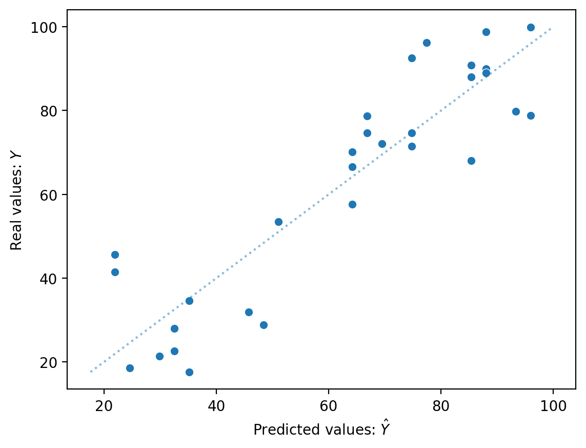
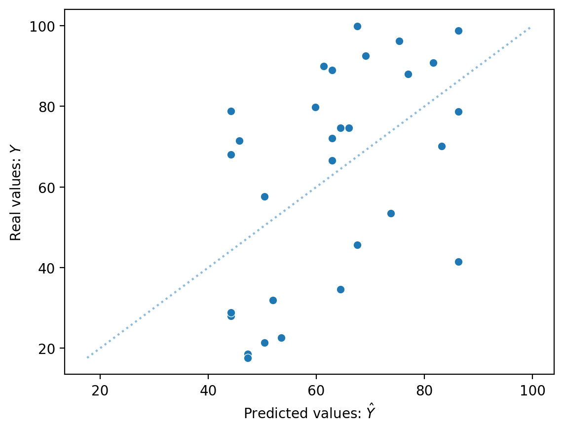
Comparing \(\hat{Y}\) to \(Y\) directly#
If we had a perfect model, \(\hat{Y}\) should be identical to \(Y\).
y_pred = mod_edu.predict()
sns.scatterplot(x = y_pred, y = df_income['Income'])
sns.lineplot(x = df_income['Income'], y = df_income['Income'], alpha = .5, linestyle = "dotted")
plt.xlabel("Predicted values: $\hat{Y}$")
plt.ylabel("Real values: $Y$")
Text(0, 0.5, 'Real values: $Y$')
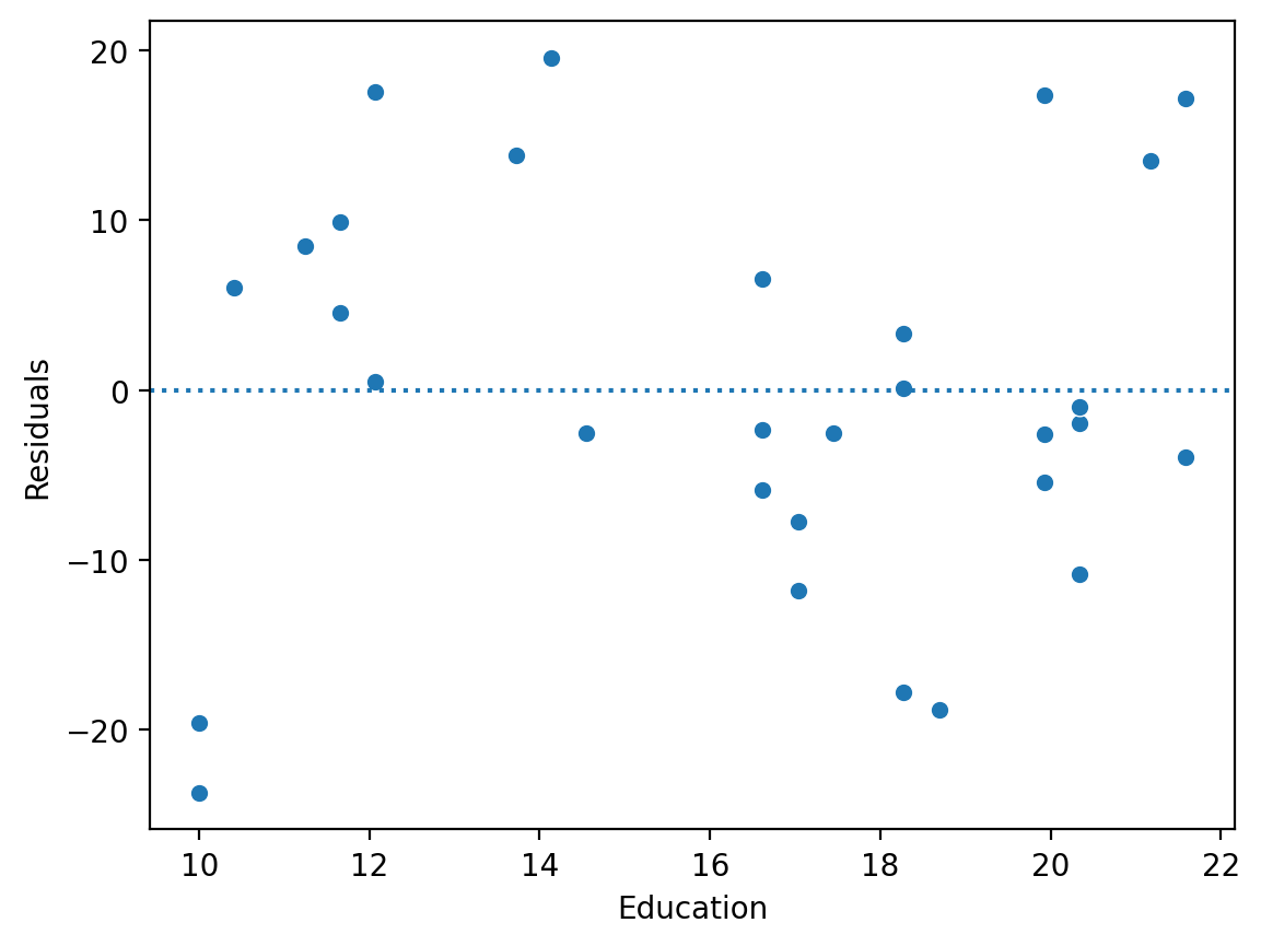
Plotting residuals#
The residuals of a model are the difference between each predicted value \(\hat{Y}\) and real value \(Y\).
We can calculate the residuals directly: \(\hat{Y} - Y\).
Or we can access them using
mod.resid.
resid = y_pred - df_income['Income'].values ### calculate residuals
sns.scatterplot(x = df_income['Education'], y = resid)
plt.axhline(y = 0, linestyle = "dotted")
plt.ylabel("Residuals")
Text(0, 0.5, 'Residuals')
Check-in#
Build a linear model predicting Income from Seniority. Then, evaluate this model using one of the visual comparison methods discussed above:
Plotting \(\hat{Y}\) as the regression line over
IncomeandEducation.Directly plotting \(\hat{Y}\) vs. \(Y\).
Plotting the residuals of our model.
### Your code here
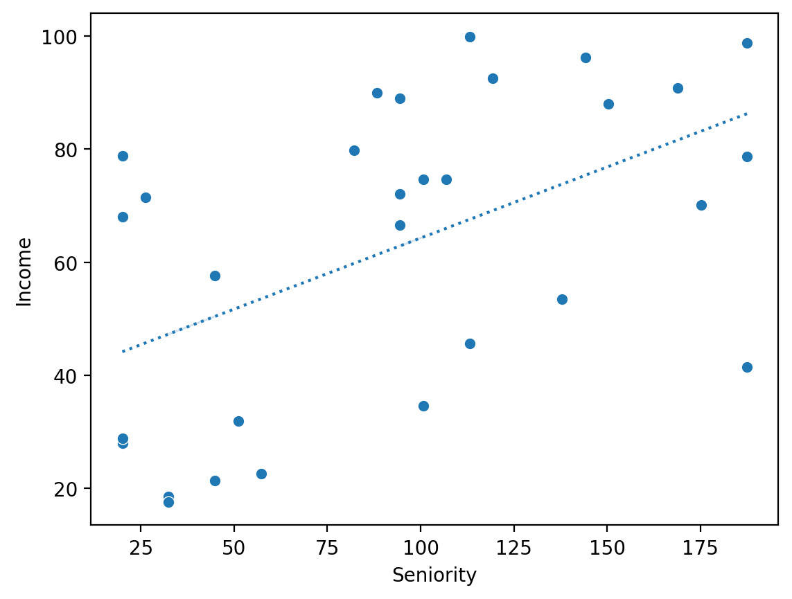
Solution (1)#
mod_seniority = smf.ols(data = df_income, formula = "Income ~ Seniority").fit()
sns.scatterplot(x = df_income['Seniority'], y = df_income['Income'])
sns.lineplot(x = df_income['Seniority'], y = mod_seniority.predict(), linestyle = "dotted")
<Axes: xlabel='Seniority', ylabel='Income'>
Solution (2)#
sns.scatterplot(x = mod_seniority.predict(), y = df_income['Income'])
sns.lineplot(x = df_income['Income'], y = df_income['Income'], alpha = .5, linestyle = "dotted")
plt.xlabel("Predicted values: $\hat{Y}$")
plt.ylabel("Real values: $Y$")
Text(0, 0.5, 'Real values: $Y$')
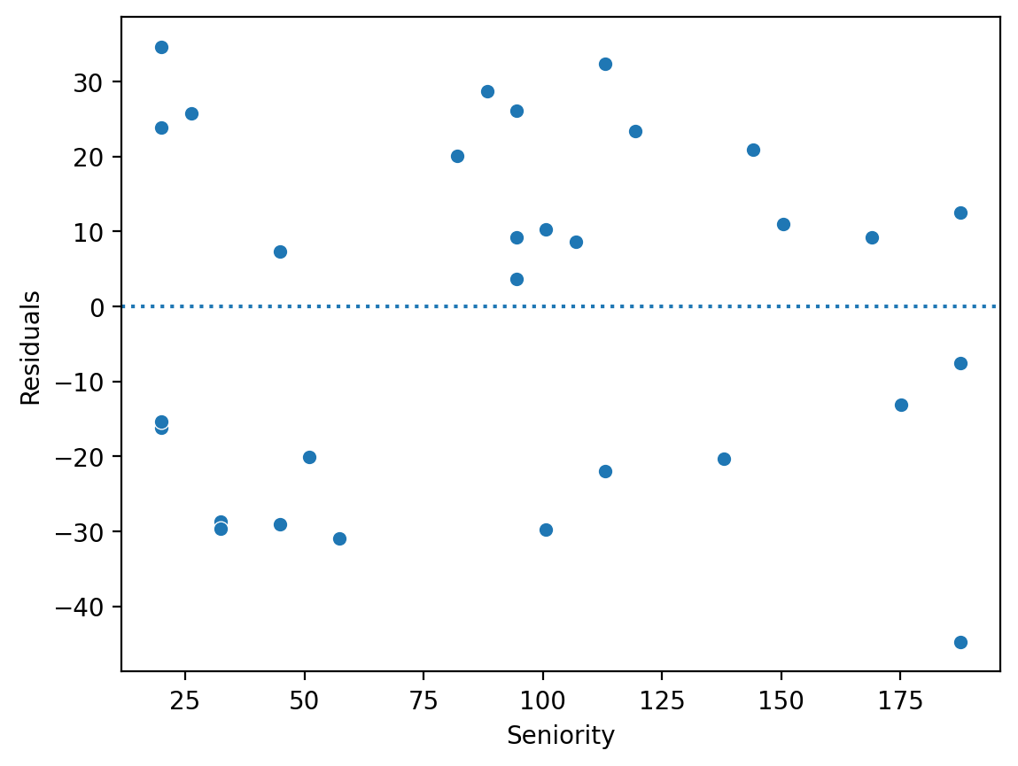
Solution (3)#
sns.scatterplot(x = df_income['Seniority'], y = mod_seniority.resid)
plt.axhline(y = 0, linestyle = "dotted")
plt.ylabel("Residuals")
Text(0, 0.5, 'Residuals')
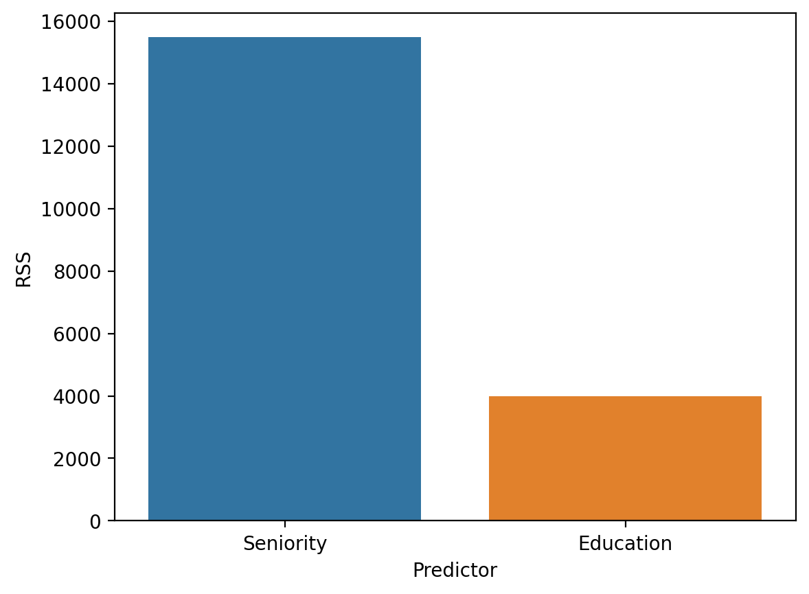
Calculating \(RSS\)#
The residual sum of squares is the sum of squared deviations between each prediction and the real values of \(Y\).
\(RSS = \sum_i^N (\hat{y}_i - y_i)^2\)
Note: A higher value is worse (i.e., more error).
### define a helper function!
def rss(y_pred, y):
    return sum((y_pred - y)**2)
## RSS for "Education" model
rss(mod_edu.predict(), df_income['Income'])
3982.506585472266
Check-in#
Calculate the \(RSS\) for your Seniority model. Is it better or worse? Does this match your intuition from the visual comparisons?
### Your code here
Solution#
## RSS for "Seniority" model
rss(mod_seniority.predict(), df_income['Income'])
15477.269661883032
Visually comparing \(RSS\)#
rss_seniority = rss(mod_seniority.predict(), df_income['Income'])
rss_education = rss(mod_edu.predict(), df_income['Income'])
df_rss = pd.DataFrame({'RSS': [rss_seniority, rss_education],
                      'Predictor': ['Seniority', 'Education']})
sns.barplot(data = df_rss, x = "Predictor", y = "RSS")
<Axes: xlabel='Predictor', ylabel='RSS'>
Calculating \(MSE\)#
The mean squared error is the \(RSS\) divided by the number of data points.
\(MSE = \frac{1}{N}*\sum_i^N (\hat{y}_i - y_i)^2\)
Note: A higher value is worse (i.e., more error).
### define a helper function!
def mse(y_pred, y):
    return (sum((y_pred - y)**2)) / (len(y))
## RSS for "Education" model
mse(mod_edu.predict(), df_income['Income'])
132.7502195157422
Check-in#
Calculate the \(MSE\) for your Seniority model. Is it better or worse? Does this match your intuition from the visual comparisons?
### Your code here
Solution#
## RSS for "Seniority" model
mse(mod_seniority.predict(), df_income['Income'])
515.9089887294344
Calculating \(S_{Y|X}\)#
The standard error of the estimate is a measure of the expected prediction error, i.e., how much your predictions are “wrong” on average.
\(\Large S_{Y|X} = \sqrt{\frac{RSS}{n-2}}\)
How much, on average, do we expect \(\hat{Y}\) to deviate from \(Y\)?
As before, a smaller number means better fit.
### Calculating directly
np.sqrt(rss(mod_edu.predict(), df_income['Income']) / (len(df_income) - 2))
11.926121668530007
Calculating using statsmodels#
A fit model in statsmodels also gives us a scale parameter; the square root of this parameter is \(S_{Y|X}\).
mod_edu.scale ## model variance
142.2323780525809
np.sqrt(mod_edu.scale) ## standard error of the estimate
11.926121668530005
Reporting \(S_{Y|X}\)#
We can report the standard error of the estimate by attaching it to our predictions, such as:
For an individual with \(10\) years of education, we predict a salary of \(21.96, \pm 11.93\).
Check-in#
What is the standard error of the estimate for the Seniority model? Is it higher or lower than the one for the Education model? What does this mean with respect to our prediction accuracy?
### Your code here
Solution#
np.sqrt(mod_seniority.scale)
23.510840707672212
\(R^2\): how much variance is explained?#
The \(R^2\), or coefficient of determination, measures the proportion of variance in \(Y\) explained by the model.
\(\Large R^2 = 1 - \frac{RSS}{SS_{Y}}\)
Check-in: Why is this a sensible formula for calculating the proportion of variance in \(Y\) explained by the model?
Decomposing \(R^2\) (pt. 1)#
First, consider the terms in the fraction:
\(RSS\): Leftover variance in \(Y\) after fitting the model.
\(SS_Y\): Total variance in \(Y\) (i.e., before fitting the model).
Thus, \(\frac{RSS}{SS_{Y}} = 1\) would mean the model hasn’t explained anything, while \(\frac{RSS}{SS_{Y}} = 0\) would mean there’s \(0\) leftover variance after fitting the model.
Decomposing \(R^2\) (pt. 2)#
So \(\frac{RSS}{SS_{Y}}\) gives us the ratio of leftover variance to Total variance.
This means that subtracting \(1 - \frac{RSS}{SS_{Y}}\) gives us the proportion of variance explained by the model (i.e., the inverse of the leftover variance).
\(R^2 = 0\) means the model hasn’t explained anything.
\(R^2 = 1\) means there’s \(0\) leftover variance.
Extracting \(R^2\)#
We can extract \(R^2\) directly from the fit model.
### What does this R^2 value mean?
mod_edu.rsquared
0.811806896672258
Check-in#
Extract the \(R^2\) for your Seniority model. What is it? How does it compare to the \(R^2\) for the Education model?
### Your code here
Solution#
### What does this R^2 value mean?
mod_seniority.rsquared
0.2686225757076368
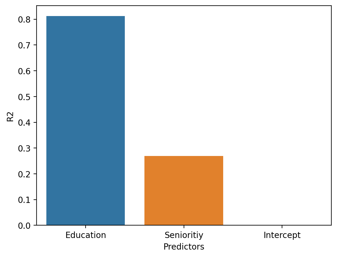
Comparing three models#
Now, let’s compare \(3\) different models:
An
Intercept-only model, i.e., with no predictors.The model with
Seniority.The model with
Education.
mod_intercept = smf.ols(data = df_income, formula = "Income ~ 1").fit()
df_r2 = pd.DataFrame({'R2': [mod_edu.rsquared, mod_seniority.rsquared,
                            mod_intercept.rsquared],
                     'Predictors': ['Education', 'Senioritiy', 'Intercept']})
sns.barplot(data = df_r2, x = "Predictors", y = "R2")
<Axes: xlabel='Predictors', ylabel='R2'>
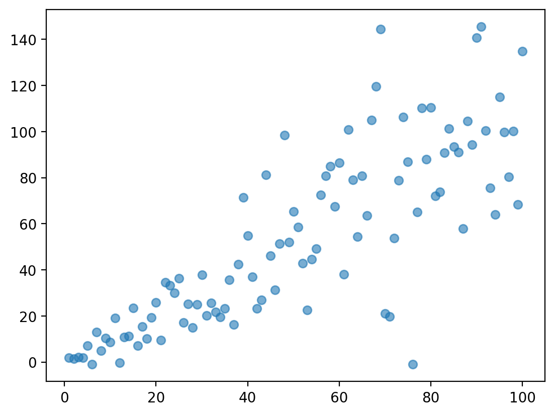
The return of heteroscedasticity#
Review: Homoscedasticity#
Homoscedasticity means that the residuals are evenly distributed along the regression line.
The opposite of homoscedasticity is heteroscedasticity.
### This is an example of heteroscedasticity
np.random.seed(1)
X = np.arange(1, 101)
y = X + np.random.normal(loc = 0, scale = X/2, size = 100)
plt.scatter(X, y, alpha = .6)
<matplotlib.collections.PathCollection at 0x173e758d0>
Check-in#
Why might heteroscedasticity pose a problem for our measures of prediction error, e.g., \(S_{Y|X}\)?
### Your answer here
Heteroscedasticity and prediction error#
The standard error of the estimate gives us an estimate of how much prediction error to expect.
But with heteroscedasticity, our error is itself correlated with \(X\).
Less error for small values of \(X\).
More error for large values of \(X\).
plt.scatter(X, y, alpha = .6)
plt.plot(X, X, linestyle = "dotted", color = "red", alpha = .6)
[<matplotlib.lines.Line2D at 0x173e76410>]

Heteroscedasticity and \(\beta\) SE#
Heteroscedasticity can also bias our estimates of the error associated with each coefficient.
Typically, this results in an underestimate of SE––potentially leading to false positives.
This is because calculating \(SE\) depends on \(S_{Y|X}\)!
Calculating \(SE(\beta)\)#
The formula for calculating the standard error of our slope coefficient is:
\(SE(\beta_1) = \frac{S_{Y|X}}{\sqrt{SS_X}} = \sqrt{\frac{\frac{1}{n-2}RSS}{SS_X}}\)
(You won’t be required to know this––but adds important context!)
Conclusion#
An important part of statistical modeling is evaluating our models, either by:
Visual inspection.
Using metrics of predictive success.
Metrics liks \(S_{Y|X}\) depend on certain assumptions being met, like homoscedasticity.