Multiple regression

Libraries

## Imports
import pandas as pd
import numpy as np
import matplotlib.pyplot as plt
import statsmodels.api as sm
import statsmodels.formula.api as smf
import seaborn as sns
import scipy.stats as ss

%matplotlib inline
%config InlineBackend.figure_format = 'retina'  # makes figs nicer!

Goals of this lecture

• Regression with multiple predictors: why?

• Implementing and interpreting models with multiple predictors.

• Techniques for identifying (or selecting) important predictors.

• Models with interactions.

Why multiple regression?

Multiple regression means building a regression model (e.g., linear regression) with more than one predictor.

Why might we want to do this?

The curious case of ice cream sales and shark attacks

Many datasets find a correlation between the number of ice cream sales in a given month and the number of shark attacks in that month.

df_sharks = pd.read_csv("data/models/shark_attacks.csv")
df_sharks.head(1)

	Year	Month	SharkAttacks	Temperature	IceCreamSales
0	2008	1	25	11.9	76

Comparing IceCreamSales to SharkAttacks

sns.lmplot(data = df_sharks, x = "IceCreamSales", y = "SharkAttacks")

/Users/seantrott/anaconda3/lib/python3.11/site-packages/seaborn/axisgrid.py:118: UserWarning: The figure layout has changed to tight
  self._figure.tight_layout(*args, **kwargs)

<seaborn.axisgrid.FacetGrid at 0x13f5d5790>

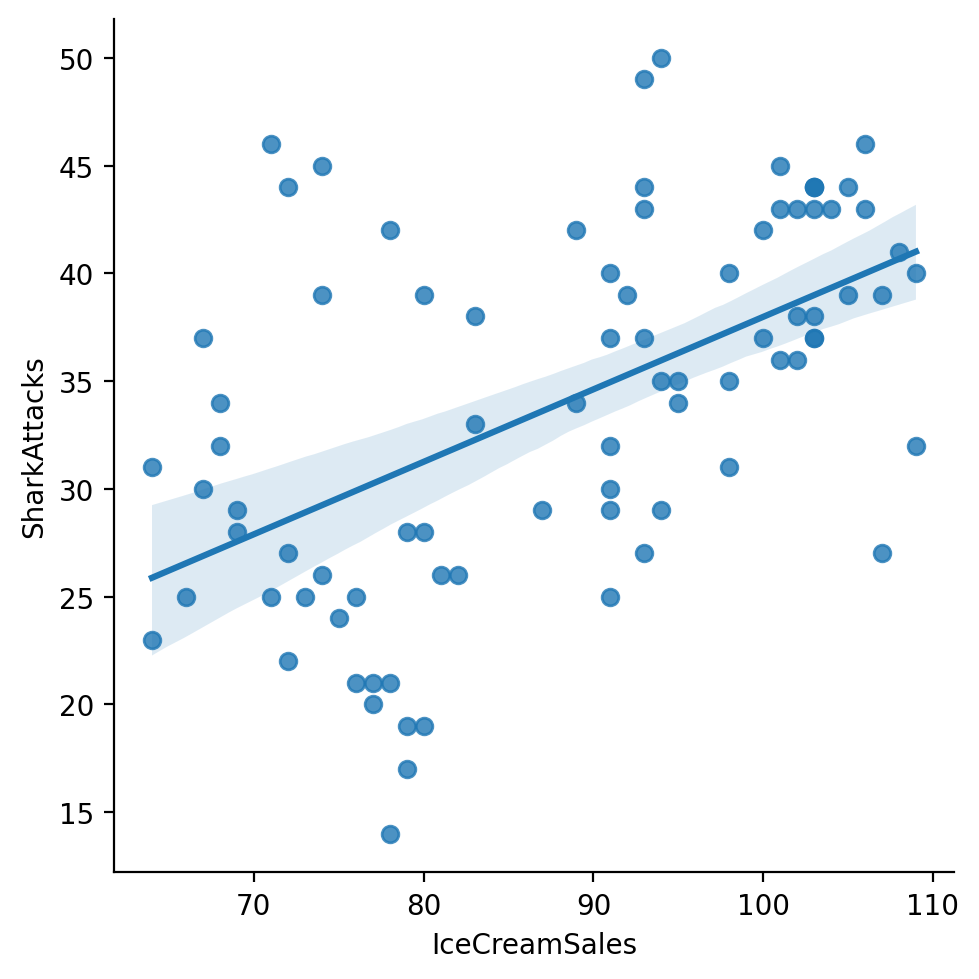
Testing with univariate linear regression

In a univariate linear model, IceCreamSales is significantly predictive of SharkAttacks (\(p < .001\)).

mod_ic = smf.ols(data = df_sharks, formula = "SharkAttacks ~ IceCreamSales").fit()
mod_ic.params

Intercept        4.352305
IceCreamSales    0.336269
dtype: float64

mod_ic.pvalues

Intercept        4.084159e-01
IceCreamSales    1.647822e-07
dtype: float64

Check-in

What other variable might be correlated with both SharkAttacks and IceCreamSales?

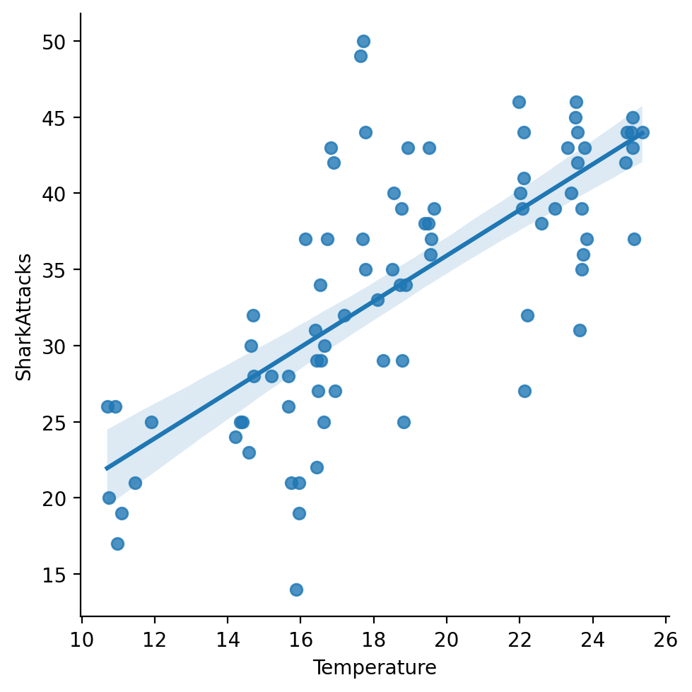
Temperature and SharkAttacks are also correlated

sns.lmplot(data = df_sharks, x = "Temperature", y = "SharkAttacks")

/Users/seantrott/anaconda3/lib/python3.11/site-packages/seaborn/axisgrid.py:118: UserWarning: The figure layout has changed to tight
  self._figure.tight_layout(*args, **kwargs)

<seaborn.axisgrid.FacetGrid at 0x13fa04e10>

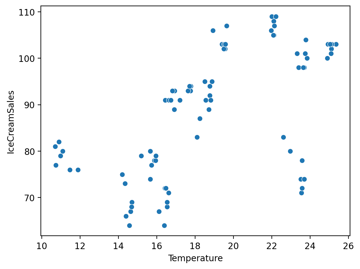
So are Temperature and IceCreamSales

(Though there also appears to be distinct clustering, possibly by Month.)

sns.scatterplot(data = df_sharks, x = "Temperature", y = "IceCreamSales")

<Axes: xlabel='Temperature', ylabel='IceCreamSales'>

Adjusting for Temperature

It’s plausible to imagine that higher temperatures have a causal impact on:

• People going to the beach (raising the likelihood of SharkAttacks).

• People buying ice cream (increasing IceCreamSales).

Thus, we can adjust for the impact of Temperature in our regression model.

mod_both = smf.ols(data = df_sharks, formula = "SharkAttacks ~ IceCreamSales + Temperature").fit()
mod_both.params

Intercept        0.565099
IceCreamSales    0.104591
Temperature      1.292756
dtype: float64

mod_both.bse

Intercept        4.305143
IceCreamSales    0.059566
Temperature      0.198021
dtype: float64

Reason 1: Adjusting for confounds

One reason to add multiple variables to a linear model is to adjust for confounding variables.

This allows you to identify the independent effect of two or more \(X\) variables on \(Y\).

Reason 2: Better models.

Typically, adding more parameters (\(p\)) improves model fit.

If your goal is to reduce errors, then more predictors will usually do this (reducing \(MSE\)).

Implementing and interpreting multiple regression models

Predicting California housing prices

• Presumably, many different factors determine the price of house.

• Rather than considering each in isolation, we can consider them together.

What factors would you like to include?

df_housing = pd.read_csv("data/housing.csv")
df_housing.head(2)

	longitude	latitude	housing_median_age	total_rooms	total_bedrooms	population	households	median_income	median_house_value	ocean_proximity
0	-122.23	37.88	41.0	880.0	129.0	322.0	126.0	8.3252	452600.0	NEAR BAY
1	-122.22	37.86	21.0	7099.0	1106.0	2401.0	1138.0	8.3014	358500.0	NEAR BAY

Using housing_median_age and median_income

To start, let’s use both the median age of houses as well as the median income in a neighborhood.

mod_housing = smf.ols(data = df_housing,
                     formula = "median_house_value ~ housing_median_age + median_income").fit()

Interpreting our parameters

With multiple regression, each coefficient \(\beta_j\) reflects:

• Amount of change in \(Y\) associated with changes in \(X_j\)…

• …holding all other variables constant (i.e., ceteris paribus).

### Interpreting parameters
mod_housing.params

Intercept            -10189.032759
housing_median_age     1744.134446
median_income         43169.190754
dtype: float64

Check-in

How would you write this as a linear equation?

Writing our model as a linear equation

With two predictors, our model looks like this:

\(Y = \beta_0 + \beta_1 X_1 + \beta_2 X_2\)

So in this case, it’d look like:

\(Y = -10189 + 1744 * X_{age} + 43169 * X_{income}\)

Interpreting the Intercept

With this equation, the Intercept is the predicted price of houses that are:

• age = 0.

• income = 0.

\(Y = -10189 + 1744 * X_{age} + 43169 * X_{income}\)

Which ends up being a negative value (weirdly).

Interpreting \(\beta_{age}\)

\(\beta_{age}\) refers to the predicted increase in a house’s price, for each 1-unit increase in age…while holding income constant!

\(Y = -10189 + 1744 * X_{age} + 43169 * X_{income}\)

Interpreting \(\beta_{income}\)

\(\beta_{income}\) refers to the predicted increase in a house’s price, for each 1-unit increase in income…while holding age constant!

\(Y = -10189 + 1744 * X_{age} + 43169 * X_{income}\)

Putting it all together

• Any given observation, of course, has both an age and an income.

• Thus, the model reflects \(\hat{Y}\) for a particular age and a particular income.

## predicted price for age = 10 and income = 10
-10189 + 1744 * 10 + 43169 * 10

438941

## predicted price for age = 20 and income = 10
-10189 + 1744 * 20 + 43169 * 10

456381

## predicted price for age = 10 and income = 20
-10189 + 1744 * 20 + 43169 * 20

888071

Evaluating our model

Typically, models with more parameters (\(p\)) have better fit, e.g., higher \(R^2\) and lower \(S_{Y|X}\).

## rsquared
mod_housing.rsquared

0.5091195899765238

## standard error of the estimate
np.sqrt(mod_housing.scale)

80853.38432785697

Check-in

Build two univariate regression models, predicting median_house_value from each of the two predictors considered below (i.e., a model for age and a model for income). What is the \(R^2\) of each of these models?

### Your code here

Solution

mod_age = smf.ols(data = df_housing,
                     formula = "median_house_value ~ housing_median_age").fit()
mod_income = smf.ols(data = df_housing,
                     formula = "median_house_value ~ median_income").fit()

print(mod_age.rsquared)
print(mod_income.rsquared)

0.011156305266713185
0.4734474918071987

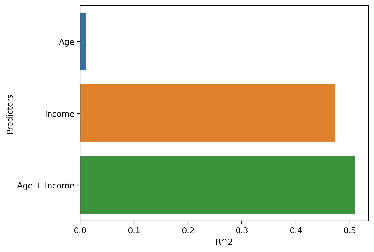
Visualizing differences in \(R^2\)

Building intuition: Based on this visualization, which variable of the two do you think seems more important? (Coming up later this lecture!)

df_r2 = pd.DataFrame({'R^2': [mod_age.rsquared, mod_income.rsquared, mod_housing.rsquared],
                     'Predictors': ['Age', 'Income', 'Age + Income']})
sns.barplot(data = df_r2, y = "Predictors", x = "R^2")

<Axes: xlabel='R^2', ylabel='Predictors'>

Models with “interactions”

Removing the additive assumption

An “interaction effect” occurs when the effect of one variable (\(X_1\)) depends on the value of another variable (\(X_2\)).

• So far, we’ve assumed that different predictors have independent and additive effects.

  • I.e., main effects of a variable \(X_1\) and \(X_2\).

• An “interaction” (or “synergistic”) effect removes that assumption.

  • In model, allows for interaction \(X_1 X_2\).

Examples of common interactions

Interaction effects are often easiest to observe and understand between two categorical variables.

• Treatment x Gender: Treatment works in males but not females.

• Brain Region x Task: double dissociation between Region of damage and which Task impairment is observed on.

• Food x Condiment: enjoyment of a Condiment depends on kind of food.

  • E.g., Ketchup is good on Hot Dog, while Chocolate Sauce is good on Ice Cream.

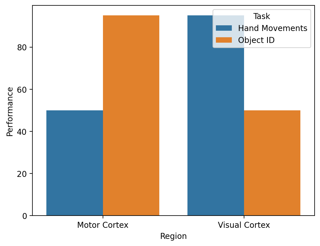
Double dissociations

In neuroscience, a double dissociation is a demonstration that two brain areas (or biological systems) have independent or localizable effects.

df_damage = pd.DataFrame({'Region': ['Motor Cortex', 'Motor Cortex', 'Visual Cortex', 'Visual Cortex'],
                         'Task': ['Hand Movements', 'Object ID', 'Hand Movements', 'Object ID'],
                         'Performance': [50, 95, 95, 50]})
sns.barplot(data = df_damage, x = "Region", 
            y = "Performance", hue = "Task")

<Axes: xlabel='Region', ylabel='Performance'>

Discovering interactions with data visualization

As a first illustration of an interaction between categorical and continuous variable, let’s consider the mtcars dataset.

df_cars = pd.read_csv("data/models/mtcars.csv")
df_cars.head(3)

	model	mpg	cyl	disp	hp	drat	wt	qsec	vs	am	gear	carb
0	Mazda RX4	21.0	6	160.0	110	3.90	2.620	16.46	0	1	4	4
1	Mazda RX4 Wag	21.0	6	160.0	110	3.90	2.875	17.02	0	1	4	4
2	Datsun 710	22.8	4	108.0	93	3.85	2.320	18.61	1	1	4	1

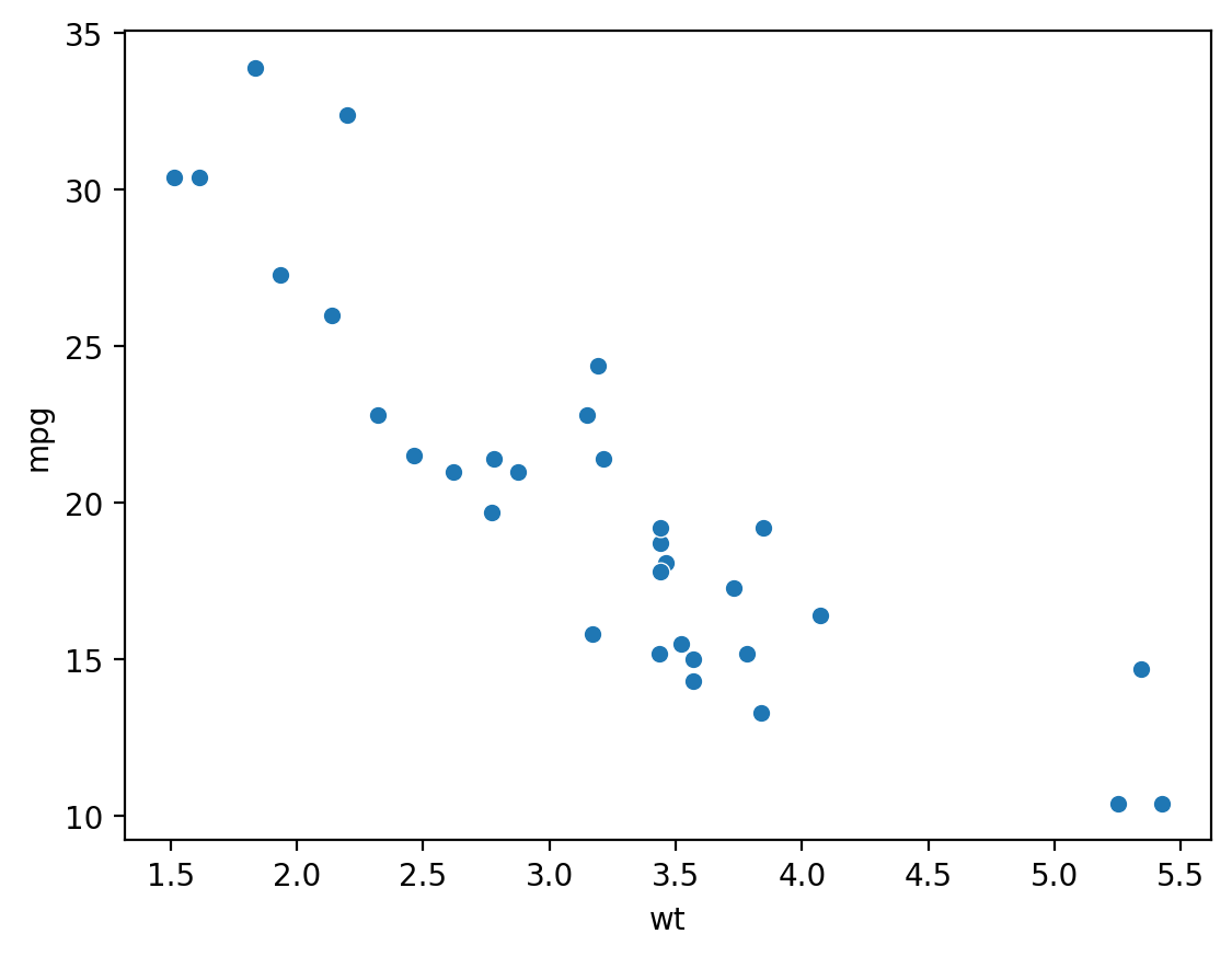
First steps: main effects (pt. 1)

This dataset contains at least two main effects: a correlation between wt and mpg, and a correlation between am (automatic = 0, manual = 1) and mpg.

sns.scatterplot(data = df_cars, x = "wt", y = "mpg")

<Axes: xlabel='wt', ylabel='mpg'>

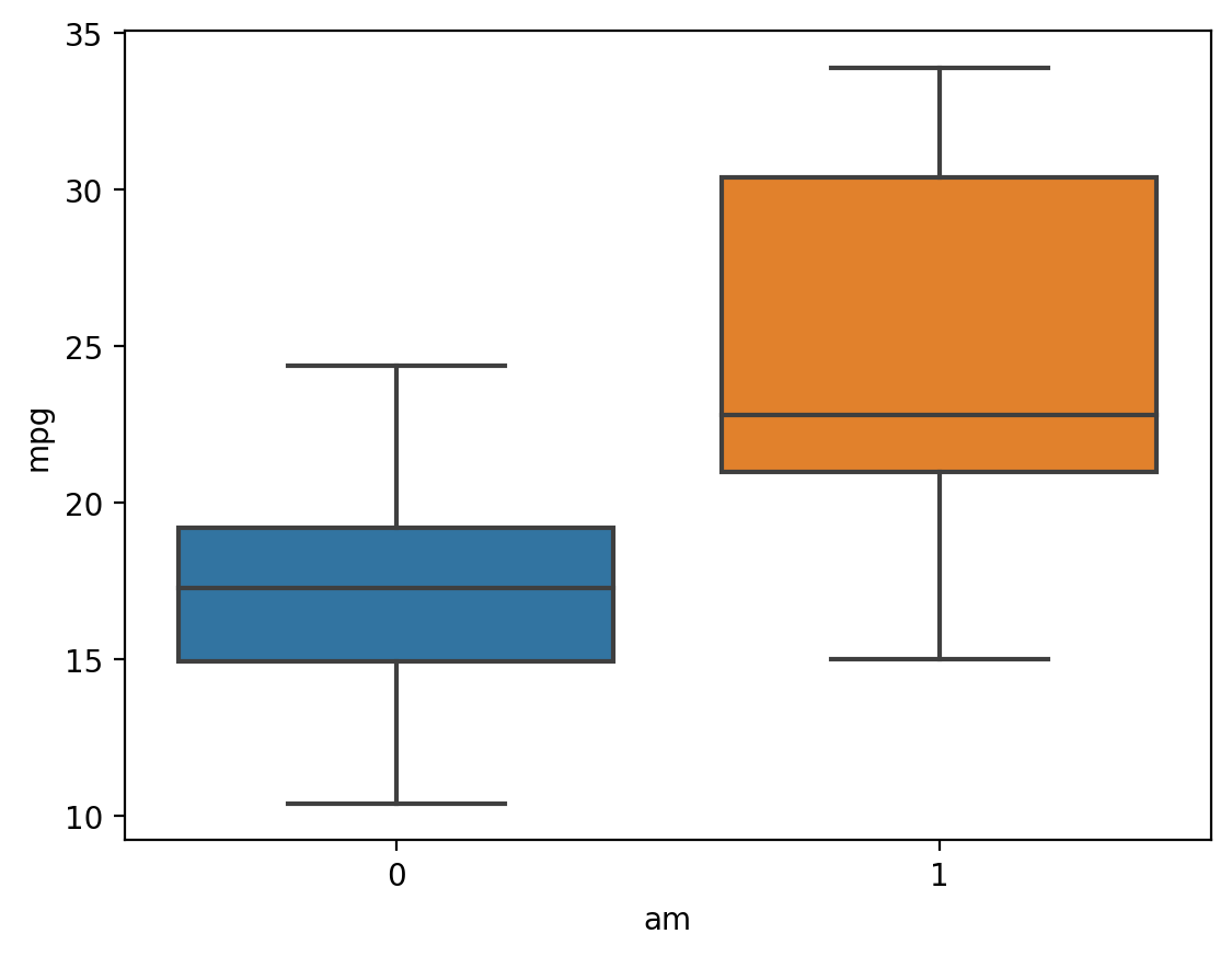
First steps: main effects (pt. 2)

This dataset contains at least two main effects: a correlation between wt and mpg, and a correlation between am (automatic = 0, manual = 1) and mpg.

sns.boxplot(data = df_cars, x = "am", y = "mpg")

<Axes: xlabel='am', ylabel='mpg'>

Check-in

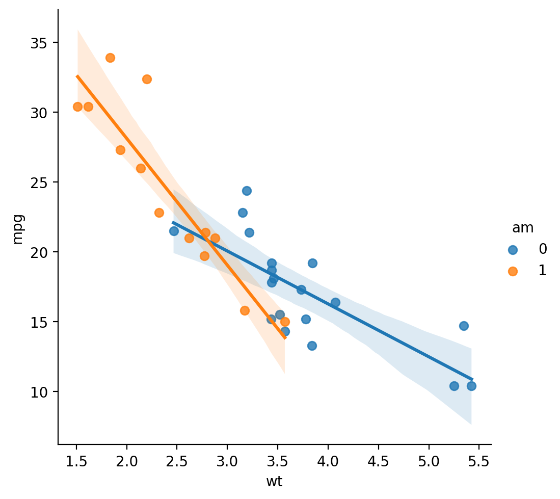
How could we use data visualization to ask whether wt and am have an interaction effect on mpg?

### Your code here

Solution

sns.lmplot(data = df_cars, x = "wt", y = "mpg", hue = "am")

/Users/seantrott/anaconda3/lib/python3.11/site-packages/seaborn/axisgrid.py:118: UserWarning: The figure layout has changed to tight
  self._figure.tight_layout(*args, **kwargs)

<seaborn.axisgrid.FacetGrid at 0x13fd1c950>

Testing for interactions with statsmodels

In statsmodels, an interaction term can be added between two variables using the * syntax (rather than +):

formula = "Y ~ X1 * X2`

Check-in

Build a linear model predicting mpg, with an interaction between am and wt. What can we conclude about the result?

### Your code here

Model output

The \(p\)-value for wt:am is significant, suggesting a significant interaction.

mod_interaction = smf.ols(data = df_cars, formula = "mpg ~ wt * am").fit()
mod_interaction.summary()

OLS Regression Results

Dep. Variable:	mpg	R-squared:	0.833
Model:	OLS	Adj. R-squared:	0.815
Method:	Least Squares	F-statistic:	46.57
Date:	Fri, 12 Jan 2024	Prob (F-statistic):	5.21e-11
Time:	10:40:17	Log-Likelihood:	-73.738
No. Observations:	32	AIC:	155.5
Df Residuals:	28	BIC:	161.3
Df Model:	3
Covariance Type:	nonrobust

	coef	std err	t	P>|t|	[0.025	0.975]
Intercept	31.4161	3.020	10.402	0.000	25.230	37.602
wt	-3.7859	0.786	-4.819	0.000	-5.395	-2.177
am	14.8784	4.264	3.489	0.002	6.144	23.613
wt:am	-5.2984	1.445	-3.667	0.001	-8.258	-2.339

Omnibus:	3.839	Durbin-Watson:	1.793
Prob(Omnibus):	0.147	Jarque-Bera (JB):	3.088
Skew:	0.761	Prob(JB):	0.213
Kurtosis:	2.963	Cond. No.	40.1

Notes:
[1] Standard Errors assume that the covariance matrix of the errors is correctly specified.

Interpreting parameters

• wt: negative slope, i.e., heavier cars have lower mpg.

• am: positive slope, i.e., manual cars have higher mpg.

• wt:am: negative slope, i.e., a stronger (steeper) effect of wt on mpg for manual than automatic cars.

\(\hat{Y} = 31.41 - 3.79*X_{weight} + 14.88*X_{am} - 5.3 * X_{weight} * X_{am}\)

mod_interaction.params

Intercept    31.416055
wt           -3.785908
am           14.878423
wt:am        -5.298360
dtype: float64

Which predictors matter?

The problem of too many parameters

• Adding more parameters will always at least slightly improve the model.

• But too many parameters can also lead to overfitting (coming up!).

• It can also make the model very hard to interpret.

• Thus, it’s important to identify which parameters are most important.

There are many approaches to identifying which parameters matter the most.

Building intuition: Comparing \(R^2\)

A visual comparison of \(R^2\) for models with different predictors helps build intuition.

What is the relative improvement in the “full” model (Age + Income) compared to each of the “simpler” models (Age vs. Income)?

sns.barplot(data = df_r2, y = "Predictors", x = "R^2")

<Axes: xlabel='R^2', ylabel='Predictors'>

Introducing subset selection

Subset selection refers to identifying the subset of \(p\) predictors that are most related to the response, i.e., result in the “best” model.

Basic logic:

• Fit a bunch of different models.

• Identify which model is best using a measure of model fit.

  • Ideally, this measure should correct for the problem of over-fitting.

Best subset selection

In Best subset selection, you fit a separate model for each combination of \(p\) predictors.

• For each parameter, fit a separate model with that predictor.

• For each pair of predictors, fit a separate model with that pair.

• … And so on.

Why might this be challenging to do in practice?

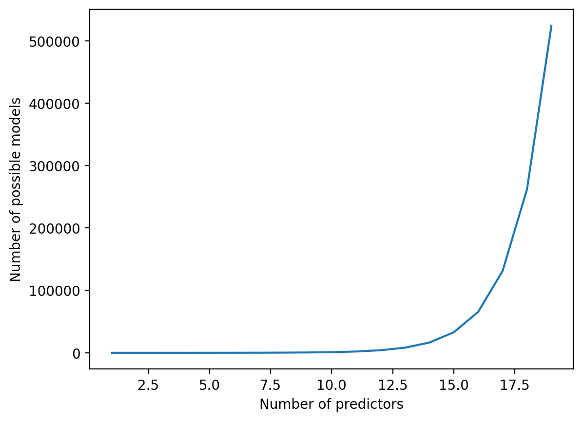
An ideal but intractable solution

As \(p\) increases, the number of possible models also increases. There are approximately \(2^p\) models considering \(p\) predictors.

p = np.arange(1, 20)
m = 2 ** p
plt.plot(p, m)
plt.xlabel("Number of predictors")
plt.ylabel("Number of possible models")

Text(0, 0.5, 'Number of possible models')

Forward selection

In forward stepwise selection, we add predictors to the model one at the time; at each time-step, we add the predictor that best improves the model.

1. Start with the “null” model (no predictors), i.e., \(M_{k=0}\).

2. Build a model for each of your \(p\) predictors. Which one is best?

3. Build a model with the single best predictor from (2), i.e., \(M_{k=1}\).

4. Repeat this iteratively, until we’ve included all predictors \(p\).

Using this procedure, the order in which predictors are added reflects how much they improve the model.

Sub-optimal, but computationally efficient

• Forward selection is much more efficient than best subset selection.

• However, the “Best” model is not guaranteed.

  • E.g., maybe the best 1-variable model contains \(X_1\), but the best 2-variable model contains \(X_2 + X_3\).

Backward selection

In backward stepwise selection, we begin with all the predictors, then take out predictors in an order that least hurts our model fit.

1. Start with the “full” model (all predictors), i.e., \(M_{k=p}\).

2. Build a model taking out each of your \(p\) predictors. Which one is best?

3. Build a new model removing the predictor from (2) that least hurt the model.

4. Repeat this iteratively, until we’ve excluded all predictors \(p\).

Using this procedure, the order in which predictors are removed corresponds to how little they help the model.

Sub-optimal, but computationally efficient

• Backward selection is much more efficient than best subset selection.

• However, the “Best” model is not guaranteed.

  • E.g., maybe the best 1-variable model contains \(X_1\), but the best 2-variable model contains \(X_2 + X_3\).

Identifying the “best” model

To perform subset selection, we need some approach to evaluating which model is “best”.

• Problem: Measures like \(R^2\), \(RSS\), etc., all improve as you add more parameters.

• We need a metric that corrects for over-fitting.

How might you go about this?

Adjusted \(R^2\): a decent workaround

• In practice, there are many approaches to correcting for a larger \(p\) (coming up soon!).

• For now, we’ll focus on adjusted \(R^2\).

\(\Large Adj. R^2 = 1 - \frac{\frac{RSS}{(n - p - 1)}}{\frac{TSS}{n - 1}}\)

Where:

• \(n\): number of observations.

• \(p\): number of predictors.

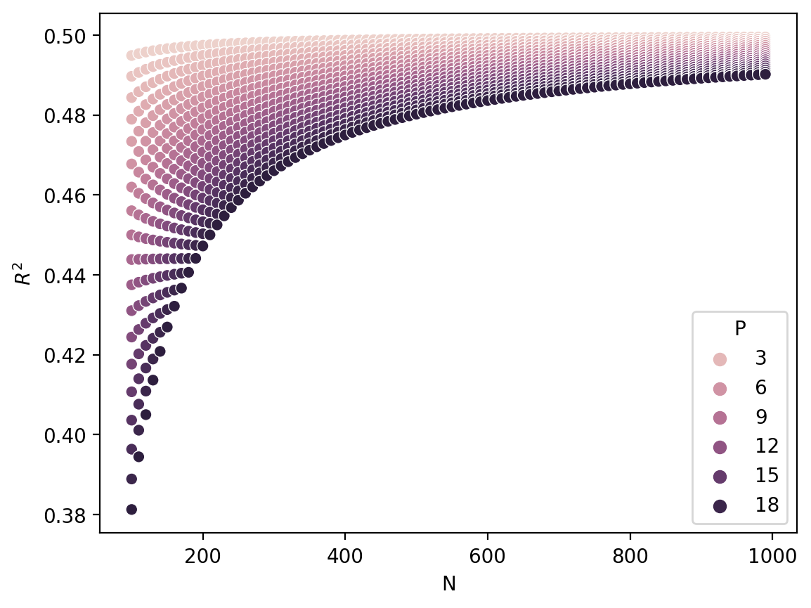
Adjusted \(R^2\): a simulation

Let’s consider a range of different models with the same \(R^2\), but different values for \(n\) and \(p\).

What do you notice about this plot?

def calculate_adj(row):
    return 1 - (RSS / (row['N'] - row['P'] - 1)) / (TSS / (row['N'] - 1))
N = np.arange(100, 1000, step = 10)
P = np.arange(1, 20)
combos = [(n, p) for n in N for p in P]
df_adj = pd.DataFrame(combos, columns = ["N", "P"])
### Suppose constant RSS and TSS
RSS, TSS = 500, 1000
df_adj['r2_adj'] = df_adj.apply(calculate_adj, axis = 1)

sns.scatterplot(data = df_adj, x = "N", y = "r2_adj", hue = "P")
plt.ylabel("$R^2$")

Text(0, 0.5, '$R^2$')

Extracting adjusted \(R^2\) from statsmodels

• We can access this value using model.rsquared_adj.

• Note that it can be negative in some cases!

mod_housing = smf.ols(data = df_housing,
                     formula = "median_house_value ~ housing_median_age + median_income").fit()
print(mod_housing.rsquared)
print(mod_housing.rsquared_adj)

0.5091195899765238
0.5090720171306622

Stepwise selection in practice

Let’s consider the case of forward stepwise selection, focusing on just these two variables predicting median_house_value.

Step 1: Null model

The null model can be fit by simply adding 1 as a predictor, i.e., an Intercept-only model.

mod_null = smf.ols(data = df_housing, formula = "median_house_value ~ 1").fit()
mod_null.rsquared_adj

4.9960036108132044e-15

Step 2: univariate models

Now, we fit a model for each of our \(p\) predictors (age and income).

Which parameter yields the biggest improvement in model fit?

mod_age = smf.ols(data = df_housing, formula = "median_house_value ~ housing_median_age").fit()
mod_income = smf.ols(data = df_housing, formula = "median_house_value ~ median_income").fit()

print(mod_age.rsquared_adj)
print(mod_income.rsquared_adj)

0.011108391530172068
0.4734219780700054

Step 3: Adding more parameters

• In step 2, we decided that median_income was the best parameter for the univariate model.

• Now we add housing_median_age.

mod_both = smf.ols(data = df_housing,
                   formula = "median_house_value ~ housing_median_age + median_income").fit()
mod_both.rsquared_adj

0.5090720171306622

Interpreting our results

• The model with both predictors explains about \(51\%\) of the variance.

• The model with age explains about \(1\%\) of the variance.

• The model with income explains about \(47\%\) of the variance.

If we had to pick just one variable, we should go with income!

print("Both parameters: {x}.".format(x = round(mod_both.rsquared_adj, 2)))
print("Age: {x}.".format(x = round(mod_age.rsquared_adj, 2)))
print("Income: {x}.".format(x = round(mod_income.rsquared_adj, 2)))

Both parameters: 0.51.
Age: 0.01.
Income: 0.47.

Conclusion

• Multiple regression allows us to:

  • Identify independent effects of our predictors.

  • Build better, more predictive models.

• We can also test for interactions between our predictors.

• There are many techniques for identifying which predictors are most “important”.

  • Includes forward and backward stepwise selection.