Linear regression in Python

Linear regression in Python#

Goals of this lecture#

Implementing linear regression in statsmodels.
Interpreting model summaries:
- Interpreting coefficients for continuous data.
- Interpreting coefficients for categorical data.

Libraries#

## Imports
import pandas as pd
import numpy as np
import matplotlib.pyplot as plt
import statsmodels.api as sm
import statsmodels.formula.api as smf
import seaborn as sns
import scipy.stats as ss

%matplotlib inline
%config InlineBackend.figure_format = 'retina'  # makes figs nicer!

Regression in Python#

There are many packages for implementing linear regression in Python, but we’ll be focusing on statsmodels.

Loading our first dataset#

df_income = pd.read_csv("data/models/income.csv")
df_income.head(3)

	Education	Seniority	Income
0	21.586207	113.103448	99.917173
1	18.275862	119.310345	92.579135
2	12.068966	100.689655	34.678727

Exploratory visualization#

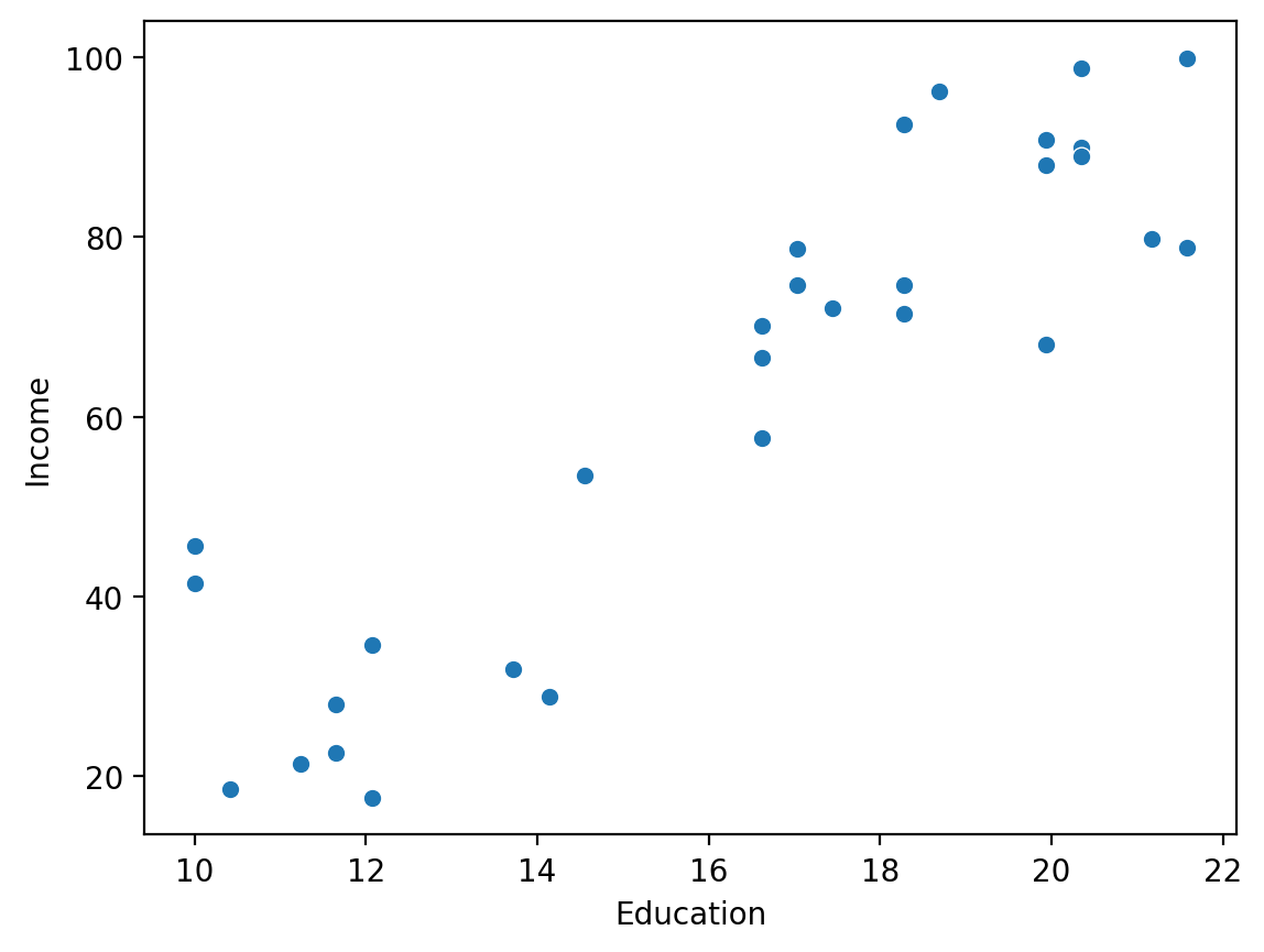
Does Education correlate with Income?

sns.scatterplot(data = df_income, x = "Education", y = "Income")

<Axes: xlabel='Education', ylabel='Income'>

../_images/3354795f7adc4e03affc5a5a75de160294a86a17f63f5615ea0c3d016e7716bc.png

Building a regression model#

We can build a regression model using statsmodels.formula.api.ols, here imported as smf.

smf.ols(data = df_name, formula = "Y ~ X").fit()

mod = smf.ols(data = df_income, formula = "Income ~ Education").fit()
type(mod)

statsmodels.regression.linear_model.RegressionResultsWrapper

Inspecting output#

mod.summary() ### Lots of stuff here!

OLS Regression Results
Dep. Variable:	Income	R-squared:	0.812
Model:	OLS	Adj. R-squared:	0.805
Method:	Least Squares	F-statistic:	120.8
Date:	Fri, 12 Jan 2024	Prob (F-statistic):	1.15e-11
Time:	10:40:11	Log-Likelihood:	-115.90
No. Observations:	30	AIC:	235.8
Df Residuals:	28	BIC:	238.6
Df Model:	1
Covariance Type:	nonrobust

	coef	std err	t	P>\|t\|	[0.025	0.975]
Intercept	-41.9166	9.769	-4.291	0.000	-61.927	-21.906
Education	6.3872	0.581	10.990	0.000	5.197	7.578

Omnibus:	0.561	Durbin-Watson:	2.194
Prob(Omnibus):	0.756	Jarque-Bera (JB):	0.652
Skew:	0.140	Prob(JB):	0.722
Kurtosis:	2.335	Cond. No.	75.7

Notes:
[1] Standard Errors assume that the covariance matrix of the errors is correctly specified.

Extracing specific information#

## coefficients
mod.params

Intercept   -41.916612
Education     6.387161
dtype: float64

## standard errors
mod.bse

Intercept    9.768949
Education    0.581172
dtype: float64

## p-values for coefficients
mod.pvalues

Intercept    1.918257e-04
Education    1.150567e-11
dtype: float64

Interpreting our model#

The linear equation#

Recall that the linear equation is written:

\(Y = \beta_0 + \beta_1 * X_1 + \epsilon\)

How would these terms map onto the coefficients below?

## Coefficients
mod.params

Intercept   -41.916612
Education     6.387161
dtype: float64

Rewriting the linear equation#

We can insert our coefficients into the equation.

\(Y = -41.92 + 6.39 * X_1 + \epsilon\)

Which can then be used to generate a prediction for a given value of \(X\).

x = 20
y = -41.92 + 6.39 * x
print(y) ### our predicted value of Y, given X!

85.88

Check-in#

Write a function called predict_y(x) which takes in a value x and outputs a prediction based on these learned coefficients.

### Your code here

Solution#

def predict_y(x):
    return -41.92 + 6.39 * x

predict_y(10)

21.979999999999997

predict_y(30)

149.77999999999997

Understanding the intercept#

The intercept term (\(\beta_0\)) is the predicted value of \(\hat{Y}\) when \(X = 0\).

What does this Intercept value mean here?

## Coefficients
mod.params

Intercept   -41.916612
Education     6.387161
dtype: float64

The intercept and the linear equation#

If \(X = 0\), the linear equation reduces to:

\(Y = -41.92 + \epsilon\)

predict_y(0) ### predicted value when x = 0

-41.92

Understanding the slope#

For a continuous variable, the slope is the predicted change in \(Y\) for every 1-unit change in \(X\).

What does this slope term mean here?

## Coefficients
mod.params

Intercept   -41.916612
Education     6.387161
dtype: float64

Check-in: more practice with `statsmodels`#

Build a regression model predicting Income from Seniority. What are the params? What do they mean?

### Your code here

Solution#

mod_seniority = smf.ols(data = df_income, formula = "Income ~ Seniority").fit()
mod_seniority.params

Intercept    39.158326
Seniority     0.251288
dtype: float64

Check-in#

Why were these parameters chosen as opposed to some other \(\beta_0\) and \(\beta_1\)?

### Your response here

Solution#

Linear regression finds the set of parameters \(\beta\) that minimizes the residual sum of squares (RSS).

I.e., it finds the line of best fit!

Other relevant output#

statsmodels also gives us:

A standard error associated with each coefficient.
A t-value associated with each coefficient.
A p-value associated with each coefficient.
A confidence interval associated with each coefficient.

Standard error#

These standard errors can be used to construct a confidence interval around our parameter estimate.
Assumption: parameters are estimates, which have some amount of normally-distributed error.

mod.bse ## Standard error associated with each coefficient

Intercept    9.768949
Education    0.581172
dtype: float64

Can report standard error as follows:

Education was positively related with Income, \([\beta = 6.34, SE = 0.58]\).

t-value and p-value#

The standard error can also be used to calculate \(t\)-statistics for each coefficient, which can in turn be used to estimate a \(p\)-value to test for significance.

## t-values = params / bse
mod.params / mod.bse

Intercept    -4.290801
Education    10.990148
dtype: float64

## double-checking our work
mod.tvalues

Intercept    -4.290801
Education    10.990148
dtype: float64

## Check for significance
mod.pvalues

Intercept    1.918257e-04
Education    1.150567e-11
dtype: float64

Check-in#

Knowing what you know about standard error of the mean, how do you think our sample size affects the standard error for our coefficients?

### Your response here

Solution#

A larger sample (\(n\)) results in a lower standard error.

Coming up soon: We’ll discuss how to actually calculate standard error for our coefficients.

Confidence interval#

Finally, the conf_int function returns a confidence interval for all of our parameters.

This is calculated using the standard error.
By default, this assumes \(\alpha = .05\), i.e., a \(95\%\) CI.
Crucial assumption is that distribution of sample statistics (\(\beta\)) is normal.

## alpha = .05
mod.conf_int()

	0	1
Intercept	-61.927397	-21.905827
Education	5.196685	7.577637

## alpha = .01
mod.conf_int(alpha = .01)

	0	1
Intercept	-68.910782	-14.922442
Education	4.781232	7.993091

Check-in#

What is the \(95\%\) confidence interval for our coefficients for the model using Seniority to predict Income?

### Your code here

Solution#

These could be reported as follows:

Seniority was positively related to Income, \([\beta = 0.25]\), \(95\%\) \(CI = [0.09, 0.41]\).

mod_seniority.conf_int()

	0	1
Intercept	21.714212	56.60244
Seniority	0.090776	0.41180

Regression with categorical predictors#

What are categorical variables?#

A categorical (or qualitative) variable takes on one of several discrete values.

Examples:

spam or not spam.
male or female.
right-handed vs. left-handed.
smoker vs. non-smoker.
treatment vs. placebo.
Condition A vs. Condition B.

Note: some variables (e.g., handnedness or gender) are treated either categorically or continuously.

Example dataset: Stroop task#

In psychology, the Stroop effect is the delay in reaction time between congruent and incongruent stimuli.

df_stroop = pd.read_csv("data/models/stroop.csv")
df_stroop.head(3)

	Condition	RT
0	Congruent	12.079
1	Congruent	16.791
2	Congruent	9.564

Building a linear model#

How do we interpret these parameters?

mod_stroop = smf.ols(data = df_stroop, formula = "RT ~ Condition").fit()
mod_stroop.params

Intercept                   14.051125
Condition[T.Incongruent]     7.964792
dtype: float64

Interpreting the slope for categorical variables#

\(\Large Y = \beta_0 + \beta_1X_1 + \epsilon\)

\(\beta_0 = 14.05\)
\(\beta_1 = 7.96\)

What is \(X_1\) here?

mod_stroop.params

Intercept                   14.051125
Condition[T.Incongruent]     7.964792
dtype: float64

Using indicator variables#

A indicator variable (alternatively: “dummy variable”) represents the possible values of a categorical variable with different numbers, e.g., 0 vs. 1 for a binary variable.

In our case, this variable might take the form:

if Condition == Congruent –> 0
if Condition == Incongruent –> 1

This is also called dummy coding or treatment coding.

Interpreting our equation with indicator variables (pt. 1)#

Our equation might thus look like this:

\(Y = 14.05 + 7.96X_{incongruent=1} + \epsilon\)

What happens when \(X\) is Congruent?
What happens when \(X\) is Incongruent?

When `Condition == Congruent`#

When Condition == Congruent, the equation reduces to the Intercept.

\(Y = 14.05 + 7.96 *0 + \epsilon = 14.05 + \epsilon\)

Note: This is actually identical to the mean of the Congruent condition!

df_stroop.groupby("Condition").mean()

	RT
Condition
Congruent	14.051125
Incongruent	22.015917

When `Condition == Incongruent`#

When Condition == Incongruent, the equation is the Intercept plus the slope.

\(Y = 14.05 + 7.96 * 1 + \epsilon = 14.05 + 7.96 + \epsilon\)

Note: The resulting value is the mean of the Incongruent condition.

14.05 + 7.96

22.01

df_stroop.groupby("Condition").mean()

	RT
Condition
Congruent	14.051125
Incongruent	22.015917

Check-in#

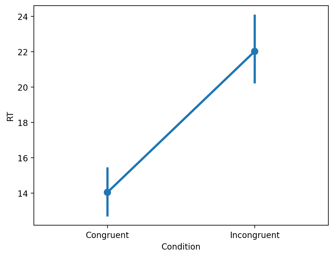
What does our slope parameter reflect then?

Solution#

In univariate regression with a categorical, binary predictor, the slope reflects the difference in means between the two levels of that predictor.

sns.pointplot(data = df_stroop, x = "Condition", y = "RT")

<Axes: xlabel='Condition', ylabel='RT'>

../_images/0ccfff9b86e2e2f7f887ad295874a5d8273ddb4c2fc4a20bd8894429c50f445d.png

Check-in#

Load the tips dataset from seaborn and fit a linear model predicting tip from time.

Inspecting the model summary.
How should you interpret the resulting coefficients?

df_tips = sns.load_dataset("tips")
### Your code here

Solution#

The intercept reflects the mean tip for Lunch, and the slope reflects the difference in tip amount between Lunch and Dinner.

mod_tips = smf.ols(data = df_tips, formula = "tip ~ time").fit()
mod_tips.params

Intercept         2.728088
time[T.Dinner]    0.374582
dtype: float64

df_tips[['time', 'tip']].groupby("time").mean()

	tip
time
Lunch	2.728088
Dinner	3.102670

Variables with \(>2\) levels?#

Many categorical variables have \(>2\) levels:

Assistant Professor vs. Associate Professor vs. `Full Professor.
Conditions A, B, and C.
Europe vs. Asia vs. Africa vs. Americas vs. Oceania.

By default, statsmodels will use dummy coding, choosing the alphabetically first level as the reference level.

Check-in#

Read in the dataset at data/housing.csv.
Then, build a linear model predicting median_house_value from ocean_proximity.
Inspect the model summary(). How should you interpret the results?

### Your code here

Solution#

df_housing = pd.read_csv("data/housing.csv")
mod_housing = smf.ols(data = df_housing, formula = "median_house_value ~ ocean_proximity").fit()
mod_housing.params

Intercept                        240084.285464
ocean_proximity[T.INLAND]       -115278.893463
ocean_proximity[T.ISLAND]        140355.714536
ocean_proximity[T.NEAR BAY]       19128.026326
ocean_proximity[T.NEAR OCEAN]      9349.691963
dtype: float64

df_housing[['ocean_proximity', 'median_house_value']].groupby("ocean_proximity").mean()

	median_house_value
ocean_proximity
<1H OCEAN	240084.285464
INLAND	124805.392001
ISLAND	380440.000000
NEAR BAY	259212.311790
NEAR OCEAN	249433.977427

How to code your variables?#

Coding refers to the approach taken to representing the different levels of a categorical variable in a regression model.

There are a variety of different approaches to contrast coding, some of which are summarized below.

Approach	Description	What is the `Intercept`?	What is the `Slope`?
Dummy coding	Choose one level as reference.	`mean` of reference group.	Difference between that level and `mean` of reference group.
Deviation coding	Compare each level to grand mean.	`mean` of all groups.	Difference between that level and grand mean.

And many more!

By default, statsmodels uses dummy coding.

Conclusion#

The statsmodels package can be used to build linear regression models.
These models produce many useful summary features, including:
- The fit \(\beta\) parameters (intercept and slope).
- The standard error and p-value of those parameters.
Each \(\beta\) parameter has a particular interpretation with respect to \(\hat{Y}\).

Linear regression in Python

Contents

Linear regression in Python#

Goals of this lecture#

Libraries#

Regression in Python#

Loading our first dataset#

Exploratory visualization#

Building a regression model#

Inspecting output#

Extracing specific information#

Interpreting our model#

The linear equation#

Rewriting the linear equation#

Check-in#

Solution#

Understanding the intercept#

The intercept and the linear equation#

Understanding the slope#

Check-in: more practice with statsmodels#

Solution#

Check-in#

Solution#

Other relevant output#

Standard error#

t-value and p-value#

Check-in#

Solution#

Confidence interval#

Check-in#

Solution#

Regression with categorical predictors#

What are categorical variables?#

Example dataset: Stroop task#

Building a linear model#

Interpreting the slope for categorical variables#

Using indicator variables#

Interpreting our equation with indicator variables (pt. 1)#

When Condition == Congruent#

When Condition == Incongruent#

Check-in#

Solution#

Check-in#

Solution#

Variables with \(>2\) levels?#

Check-in#

Solution#

How to code your variables?#

Conclusion#

Check-in: more practice with `statsmodels`#

When `Condition == Congruent`#

When `Condition == Incongruent`#